Stat 217 – Review I
To Do: In Canvas, there are two
discussion boards about Exam 1. In the
Q&A Discussion board, submit at least one question you have on the course
material. In the Sample Questions
Discussion board, suggest a possible exam question you think I could ask. Once
you post your responses you will be able to view other student responses.
Optional Review Session: Monday,
7:00-8:00pm, Office Hour Zoom Room
Exam Location: 35-111B (our lab room)
Exam Format: The exam will cover topics from Chapters
P-3 (Days 1-15; Labs 0-3, Investigations 1-4). (But not section 2.4.) The exam
questions will be a mix of multiple choice and short-answer questions, often
with several questions on the same study (but you do not necessarily have to
answer (a) to try (b) etc.). You may bring
one page of self-produced notes (8.5 x 11, double-sided). You might be
expected to use applets and describe your process and/or you could be expected
to read output (especially from One
Proportion, One
Mean, Theory-Based
Inference applets) and and/or to use your calculator and/or to set up
calculations by hand (show the values substituted into the formula). You will
be expected to explain your reasoning, indicate your steps, and interpret your
results. The exam will be worth approximately 50 points, so plan to spend one
minute per point.
Advice for Reviewing for Exam: You should study from the textbook, class
handouts, videos, quizzes, labs, investigations (including my grading
comments and the commentaries that have been added to the submission
pages). Check out the learning goals at the beginning of each section in
the text. My advice is to ask for clarifications/supplements to this material from
me rather than trying to find related material from other sources. Also
consider reviewing the reading quizzes, self-tests, and What Went Wrong
exercises found in Canvas, and the practice questions in WileyPlus.
Start with ideas we have discussed more often (e.g., observational units and
variable). Remember to work problems, not just read examples. Let me know if something is missing from the
review materials that you would like to see. In studying, I recommend going
back through (not just looking them over, but trying
to solve them from scratch on a blank piece of paper) quizzes, examples,
investigations, and labs without looking at the solutions, then checking your
answers. I also strongly recommend submitting and reviewing questions and
answers to the Exam 1 Q&A Discussion Board in Canvas (beyond the required
one minimum).
Advice for Taking the
Exam: Most problems
will have multiple parts but you do not typically have
to answer all the parts in order. If your answer does use information from an
earlier part that you did not complete, you can use an appropriate symbol in
place of that answer. If you get stuck
on a problem, move on (but don’t leave any open-ended responses blank, let me
know how far you got). Try to hit the
highlights in your answers (a 2 pt problem should
take you roughly 2 minutes) and be succinct. You might want to read all the
questions very quickly to start, to help you know which information should go
where (e.g., don’t give me the answer to (f) in part (e)). Then read each question carefully (and all
possible answer choices) before you answer.
Show all of your work and explain yourself
(some points are for communication).
Review problems Problems Solutions
These are
intended to cover the topics below and have been updated a bit to reflect more
“reading of output” than “producing of output.” Most of the questions are
open-ended but you should expect more multiple choice on the exam, though
perhaps with some “explain why that is the correct answer.” This collection of
questions is not intended to convey information about the length of the
exam. I strongly recommend working on the problems yourself and then checking
your answers rather than only reading the answers.
From the Preliminaries chapter you
should be able to:
·
Define
probability in terms of long-run relative
frequency (proportion)
o
If
asked to “define” probability don’t use the words probability, chance, likelihood,
or odds or other synonymous.
o
Make
sure you clearly indicate the random process being repeated and the outcome(s)
of interest
·
Identify
observational units (the person or object for which we record information) for
a study
o To help identify the observational units,
think about how many observations/pieces of data you have
·
Define
the variable of interest (characteristic varying from observational unit to
observational unit)
o
Make
sure you can state these as variables for the specified observational units
(e.g., hair color or whether or not have red hair)
o Don’t confuse variables with groups of
people (red heads or those with black hair)
o Don’t confuse variables with “results”
(the proportion of students with red hair)
o Don’t confuse variables with research
question (are there fewer red heads among males?)
o
Try
to specify variable as a question we can “ask” each observational unit (what is
your hair color?)
·
Classify the variable type as quantitative or
categorical
·
Describe
the behavior of a distribution (quantitative
variable: shape, center, variability, unusual observations) in context and
suggest explanations for unusual behavior
·
Anticipate
variable behavior (e.g., hair cut prices vs. number of siblings)
From Chapter 1 you should
be able to
·
Construct
and interpret a bar graph
·
Identify
the sample size (n)
·
Distinguish
between parameter (numerical summary of population or process) and statistic
(numerical summary of sample)
o
Be
able to use appropriate symbols to refer to these
o Differentiate between proportion and percentage (often you can
use either, but make sure you identify them consistently, e.g., don’t say the
proportion is 30%).
·
Define
a parameter or a statistic (in words and/or recognize the value)
·
Understand
the concept of a simulation model (replicating a
study under specific conditions, e.g., the null hypothesis is true)
·
Use
the One Proportion applet to carry out a simulation of n trials with probability of “success” ![]()
o
Be
able to indicate the input values for the boxes
o
Be
able to map out the simulation parallels to the original study (e.g., what do
heads represent, how many coin tosses, what assuming)
o
Identify
the “observational units” and “variable” of the null distribution (how would
you create another dot? What is the horizontal axis label?)
o
Be
able to anticipate some aspects of the behavior of the null distribution (e.g.,
where it will be centered)
o
Use
the output to describe typical and atypical values for the statistic when the
null hypothesis is true
o
Be
able to use applet output to estimate the p-value
·
Be
able to roughly approximate the p-value yourself based on a graph of simulated
statistics (are you in the tail of the distribution so small p-value or not)
o
Be
able to interpret the p-value in the
context of the research question
·
What
is the p-value the probability of? What
does it mean to be a probability?
·
Use
the estimated p-value to make a conclusion about the research conjecture (vs.
the by chance alone hypothesis)
o Be able to explain the logic/reasoning
behind the decision (e.g., is it likely to have obtained our observed statistic
by chance alone = when null hypothesis is true)
·
State
null and alternative hypotheses about a general process probability (the parameter)
o
Using
symbols and/or words
o
Null
hypothesis has the form: parameter equals value
§
May
what a hypothesized value other than 0.50.
o
Including
a “less than” alternative and a “not equal to” alternative, based on the
research question
§
Understand
idea of two-sided p-value considering evidence in either direction
·
Decide
whether results are statistically significant, especially given a level of
significance
o
Decide
whether to reject or fail to reject the null hypothesis
·
Standardizing
an observation (observation-mean)/SD as a way to
measure distance and how far in the tail of the distribution the observation is
o
Interpret
as number of standard deviations above or below the mean (positive or negative
values)
o
Consider
values more than 2 or 3 standard deviations from the mean as “in the tail” of
the distribution
§
A z
of 2 roughly corresponds to a two-sided p-value below .05
·
Section
1.4: Explain factors that impact strength of evidence (sample size, distance
between observed and hypothesized, one-sided vs. two-sided)
·
Section
1.5: Apply the theory-based approach for one proportion (“one-sample z-test”)
o
Calculate
and interpret the theoretical standard deviation of sample proportions: ![]()
o
State
and check the validity conditions for the normal distribution model to
reasonably predict the null distribution
§
This
includes “large population” (otherwise the SD formula might be a bit off)
o
Which
p-value in the output is considered the “theory-based p-value”
o
NO
change in how we interpret or evaluate the p-value we find
From Chapter 2 (Sections
2.1 and 2.2) you should be able to
·
Identify
the population of interest in a research study
·
Identify
and distinguish between the population (entire group of observational units of
interest) vs. the sample (those observational units from the population we
record information for)
o
Parameter
as a numerical summary of a population
o
Symbols
for statistics vs. parameters (see symbol chart in Day 12 handout? Also below)
·
Identify
the cause and direction of bias in a biased sampling method
o
How
can you tell a sampling method is biased from a distribution of sample
statistics?
o
Identify
common sources of sampling bias (e.g., voluntary response, incomplete sampling
frame)
·
Be
able to identify/describe a sampling frame
·
Discuss
how to use a sampling frame to select a simple random sample (SRS)
o
Specify
a sampling frame in a particular context (i.e., the physical list of members of
population like the phone book)
o
Number
the units in the frame, use a random number mechanism to generate ID numbers,
report the members of the sample
·
Explain
the purpose of random sampling (produce a sample representative of population)
o
Allows
us to assume there is no “sampling bias” but still may be some “random sampling
error” (by chance alone) or “nonsampling concerns”
(See Video 2.1.9)
o Long-run mean of sample statistics will
be equal to the population parameter
o Allows you to generalize
conclusions (significant or not!) from the sample to the population
·
Discuss
how results from sample to sample vary from “random sampling error” (by random
chance from the random sampling process)
·
Discuss
how the amount of “random sampling error” depends on the sample size
o
Larger
samples are more precise = statistics
cluster more closely around the parameter
o
Does
not depend on the population size as long as the
population size is much, much larger than the sample size (20x)
·
Interpret
a histogram or dotplot/ compare distributions of
quantitative data
o Eyeball the center and spread of the
distribution, identify shape as roughly symmetric, skewed right, skewed left,
or other
o
Interpret
mean as a measure of center (include measurement units)
o
Interpret
standard deviation as a measure of variability (include measurement units)
·
Be
able to compare (or conjecture) how the spread of two distributions compares
from the graphs/nature of variables involved
o
Always
put your comments into the context of the study
·
Decide
which graphs (bar graph vs. dotplot/histogram) to use
with which type of variable (categorical vs. quantitative)
·
Assess
the statistical significance of an observed sample mean based on the null
distribution
o
State
null and alternative hypotheses about m
o
Explain
what determines each of the shape, center, and variability of the null
distribution of sample means
o
Calculate
and interpret the standard error of the sample mean SE(![]() )
)
·
Expected
sample to sample variation in the sample means
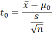
o
Calculate
and interpret the standardized statistic (t-statistic)
o
Determine
whether a distribution of sample means is expected to be normal or
approximately normally distributed
o
If
validity conditions are met, can use Theory-Based Inference applet to obtain
p-value (“one-sample t test”)
·
Identify
common sources of nonsampling concerns (e.g., poorly
worded questions, value-laden questions, social expectation, influence of
interviewer, ordering of questions, timing of study)
o
Consider
possible preventions (e.g., interviewer training, consistency, ensure
confidentiality)
From Chapter 3 you should
be able to:
·
Confidence Intervals: Determine
a range of plausible values for the “population” parameter (![]() or m)
or m)
o
All
values of parameter that would not be rejected by a two-sided test of
significance for a specified level of significance (1-confidence level)
·
Obtain
and interpret value of standard error of distribution of sample proportions SE(![]() )
)
o
From
applet (assuming some value for ![]() , can use 0.50 if nothing else)
, can use 0.50 if nothing else)
o
Using
formula ![]()
§
Understand
that sample size affects variability of sample proportions
·
Approximate
a 95% confidence interval using the “2SD Method”
o
For
95% confidence and categorical data, can approximate with ![]() + 2 SE(
+ 2 SE(![]() )
)
o
For
95% confidence and quantitative data, can approximate with ![]() + 2 s/
+ 2 s/![]()
·
Be
able to interpret confidence interval
(e.g., from output)
o
I’m
95% confident that…
o
Discuss
whether/how sample size affects confidence interval (midpoint, width)
o
Discuss
whether/how sample statistic affects confidence interval (midpoint, width)
o
Discuss
whether/how confidence level (e.g., 95%) affects confidence interval (midpoint,
width)
o
Define
margin-of-error (half-width of interval, the “plus or minus” part)
§
What
it measures (and what it does not measure)
·
Categorical
data: Can use Theory-Based Inference applet to obtain confidence interval based
on normal null distribution (“one-sample z
interval”)
o
Given
summary data or data file
o
Need
large sample size (at least 10 successes and at least 10 failures in the
sample) for this approach to be considered valid (and large population)
o
Or
use the Plus Four method, adding 2 successes and 2 failures to the data set
before asking the computer to find the interval
·
Quantitative
data: Can use Theory-Based Inference applet to obtain confidence interval based
on normal null distribution (“one-sample t interval”)
o
Given
summary data or data file
o
Need
large sample size (at least 20 in the sample) or normally distributed
population for this approach to be considered valid (and large population)
·
Interpret
confidence level
o
By
“95% confidence” I mean 95% of the time…
·
Section
3.4: Explain factors that influence the width of a confidence interval
Some general notes
·
Be
able to define parameter as a process probability or a population proportion or
a population mean or a “long run mean” (sometimes you know their numerical
value, sometimes you just describe in words what the unknown number represents)
·
Don’t
overuse the word “bias”
o
Bias
is not just being wrong, but repeated samples producing statistics that are consistently
wrong in a particular direction
o
Don’t
try to list all possible sources of bias but focus on one primary source
o
Be
sure to specify and justify the direction
of the bias (do you suspect the sampling method will lead to a tendency to
over- or under-estimate the parameter of interest?)
o
Remember
that increasing the sample size does NOT get rid of “sampling bias” (just ask
folks at the Literary Digest magazine)
§
Can
say it reduces the amount of “random sampling error”
·
Be
able to explain the overall reasoning of “statistical significance”
o
Can
we plausibly eliminate “random chance” as an explanation for our statistic?
§ What is the goal of the simulation?
§ How is the simulation carried out?
§
What
can you predict in advance about the simulation results?
§
How
do we compute the p-value?
§
How
do we interpret the p-value (“under the assumption that…”)
§
How
do we draw conclusions from the simulation results?
·
Be
able to use the applets or fill in information in applet screens
·
Know
the difference between a question asking you to interpret a p-value and one asking you to evaluate a p-value or make a decision
based on the size of the p-value. (Similarly for standardized statistic)
·
When
making statements/conclusions, always cite relevant graphical and numerical
support when possible
·
Don’t
say words like “random” or “normal” or “significant” or “variability” or “range” or “confident” unless you
really mean their technical definitions
Symbols:
|
|
Categorical variable |
Quantitative variable |
|
Parameter |
|
|
|
Statistic |
|
|
|
Graph |
bar graph |
histogram, dotplot |
|
Null
hypothesis |
H0: |
H0: |
|
Shape
of null distribution |
approximately normal if sample size large
(at least 10 successes and at least 10 failures in sample) |
normal if population
is normal OR approximately normal is sample size large (n > 20) |
|
Mean
of null distribution |
Hypothesized
probability |
Hypothesized
mean |
|
Standard
deviation of statistic |
SD of |
SD of |
|
Standard
error of statistic |
SE of |
SE of |
|
Approximate
95% margin
of error |
2 × |
2 × s/ |
|
Standardized
statistic |
|
|
|
Confidence
interval |
With Plus
Four Method, add 2 successes and 2 failures first. |
|
Notes:
- “Standard error” just means it’s an estimate of a theoretical
standard deviation. You can pretty much ignore this distinction and just
think in terms of standard deviation.
Read “SD(
 )” as “standard deviation of ” (one number).
  0 and
0 and  0 are symbols referring to the
hypothesized values of the parameters.
They are what we compare to when standardizing our statistic.
0 are symbols referring to the
hypothesized values of the parameters.
They are what we compare to when standardizing our statistic.