Stat
217 Review 1 Problem Solutions
1) a. Blood type - categorical
b. Waiting time – quantitative (if recorded as number of
minutes between arrival and seen by doctor).
c. Mode of arrival (ambulance, personal car, on foot, other) -
categorical
d. Whether or not men have to wait longer than women – this is
a research question/comparison, not a variable posed to individual visitors
(the variables asked of the visitors would be length of wait and gender)
e. Number of patients who arrive before noon – this is a
summary of the data, not a variable posed to individual visitors, the variable
would be whether or not the patient arrived before noon
f. Whether or not the patient is insured - categorical
g. Number of stitches required – quantitative
h. Whether or not stitches are required - categorical
i. Which patients require stitches – a subgroup of the sample,
not a variable posed to individual visitors (see g and h)
j. Number of patients who are insured – this is a summary of
the data, not a variable posed to individual visitors (see f)
k. Assigned room
number – categorical (numerical but doesn’t make sense to talk about “average”
room number)
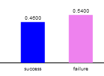
2) a. A bar graph showing the proportion that landed up
(success) and the proportion that landed down (failure):
b. The
parameter of interest is the underlying long-run probability of a spun racquet
landing up.
c. Null
hypothesis: the probability of landing up is .50 (![]() =
.5)
=
.5)
Alternative hypothesis:
the probability of landing up is not .50 (![]()
![]() .5)
.5)
We are using a
two-sided alternative hypothesis because we wouldn’t want to use this method to
see who serves first if either the
racquet lands up more than half the time or
if it lands up less than half the time.
d. Flip a coin
100 times and record the time of times the coin lands heads. Let this represent the racquet landing
“up.” Repeat this process a large number
of times and look at the distribution of the number of heads across all these
trials. Then see where 46 falls in this
distribution. If it falls is in the tail
of the distribution, we have evidence that the racquet was not landing equally
heads/tails in the long-run. If 46 falls
among the “typical” values in this distribution, then we don’t have evidence
against the belief that the racquet is 50/50 when spun this way.
e. The graph
that is centered at 0.50, our hypothesized probability of success is the
correct one (the one on the left).
f. From this
output, we see that 0.46 is not unusual for a 50/50 coin. Therefore, we would
not consider a result of 46 “ups” and 54 “downs” to be surprising if the
racquet spinning truly was a 50/50 process.
We do not have convincing evidence that this is not a 50/50 process.
To calculate a
p-value here, we would consider results “or more extreme” to be those further
away from 50 in either direction. We
would see how often we got 46 or fewer heads OR 54 or more heads (aka 46 or
fewer tails). Adding these together
would give us our p-value.
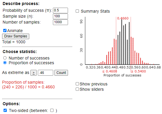
Two-sided simulation-based p-value = 0.4660 This is not a small p-value
(e.g, .466 > .05), so we fail to reject the null hypothesis.
3) a. The population is all Cal Poly students and the sample
is the 97 who responded.
b. The
parameter is the proportion of all Cal Poly students who eat breakfast 6 or 7
times a week. We could call this (unknown) value ![]() . The statistic is the proportion of the
sampled students who report eating breakfast 6 or 7 times a week. We know the
second number to be
. The statistic is the proportion of the
sampled students who report eating breakfast 6 or 7 times a week. We know the
second number to be ![]() = 35/97 = .361.
= 35/97 = .361.
Note: .21 is
the population proportion at James Madison, not ![]() or
or ![]() .
.
|
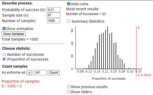
To find the p-value,
we can consider two approaches, simulation and theory-based. For the
simulation approach we can use the One Proportion applet (note we are
assuming the population here is much larger than the sample, more than 20
times larger). We want to set the sample size to be 97 and we are going to
conduct the simulation assuming the proportion of all Cal Poly students is also .21 as it was at James Madison
University. Then we see how often random samples from such a population yield
a sample proportion of .361 or higher (the direction conjectured by the
researchers).
Alternatively,
we could consider using the normal approximation because there were 35
“successes” and 62 “failures,” both at least 10, so the approximation should
be valid. Using the Theory-Based Inference applet
We again find
a very small p-value. In addition, this applet tells us that our observed
statistic ( |
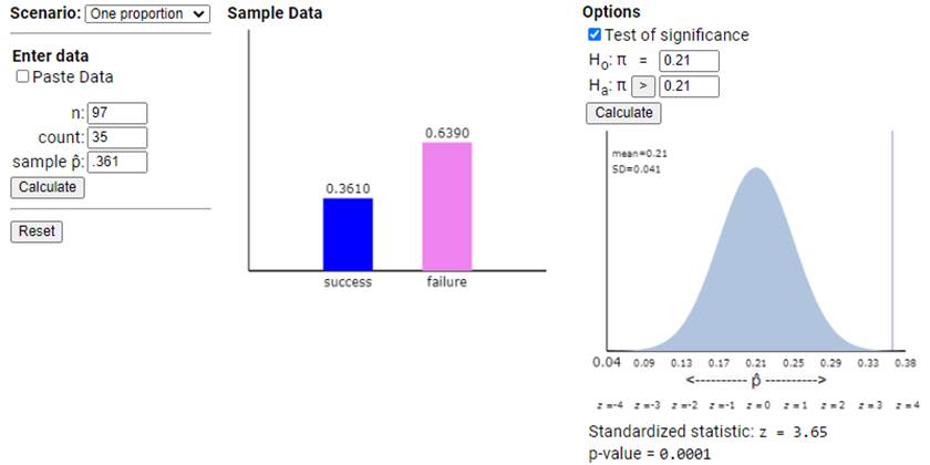
c. The p-value
is clearly small (.001 < .05), so we reject the null hypothesis that ![]() , the proportion of all Cal Poly
students who eat breakfast 6 or 7 times as week, equals .21, in favor of the
alternative the hypothesis that
, the proportion of all Cal Poly
students who eat breakfast 6 or 7 times as week, equals .21, in favor of the
alternative the hypothesis that ![]() > .21.
Thus, we conclude that there is convincing evidence that more than 21%
of all Cal Poly students eat breakfast 6 or 7 times a week. So at least on this
measure of “healthiness” we have strong evidence that the Cal Poly population
is healthier.
> .21.
Thus, we conclude that there is convincing evidence that more than 21%
of all Cal Poly students eat breakfast 6 or 7 times a week. So at least on this
measure of “healthiness” we have strong evidence that the Cal Poly population
is healthier.
d. The p-value
says that if we were to repeatedly take simple random samples of 97 students
from a population with ![]() =
.21, then in less than .1% (depending what you find for the p-value) of those
samples would we find our sample proportion
=
.21, then in less than .1% (depending what you find for the p-value) of those
samples would we find our sample proportion ![]() who eat
breakfast at least 6 times a week to be .361 or higher.
who eat
breakfast at least 6 times a week to be .361 or higher.
e. The
statistic (![]() ) will probably be different but not the parameter (
) will probably be different but not the parameter (![]() ).
The population parameter is a fixed (but unknown to us) value.
).
The population parameter is a fixed (but unknown to us) value.
f. This indicates
a potential source of sampling bias. Those who chose to respond to the survey
could be different from those who did not.
Perhaps they are more aware of their eating habits and more interested
in health overall and that’s why they were more likely to reply, leading to an
overestimate of the population proportion in this study.
g. We need a
list of all Cal Poly students (the sampling frame) probably from the
registrar’s office. Assign everyone on
the list a unique 5 digit number. Then
use a random number table or computer or calculator to randomly select 1590
unique ID numbers. Find and survey those
students.
h. If there is
still a high nonresponse rate, even with the larger sample size we would still
be concerned about how representative the sample is. It would be much, much better to recontact
the originally selected people (several times if necessary) to get their
responses than to simply sample more people.
i. With the
larger sample size and the same value for the statistic we would expect the
p-value to be even smaller. The sampling
distribution of the sample proportions (![]() ’s) would cluster even closer around .21 (less
sampling variability) and it would be even more shocking to randomly obtain a
sample proportion as extreme as .361 when
’s) would cluster even closer around .21 (less
sampling variability) and it would be even more shocking to randomly obtain a
sample proportion as extreme as .361 when ![]() =
.21.
=
.21.
4) a. The sample size was 100
and had 46 up and 54 down, both above 10. So yes, we would predict a normal
shape to the distribution of sample proportions.
b. We are 95% confidence that the probability a
spun racquet lands heads is between .3656 and .5575. That is, if we spin the racquet forever, then
in the long run we expect between 36.6% and 55.8% to land up.
c. The confidence interval should get narrower
(less wide) with the larger sample size.
d. Well, we can’t say this for sure, but we can
say .5 is a plausible value for the probability of landing up because .5 is
captured inside our 95% confidence interval. In other words, it’s plausible
that if we repeatedly spun this racquet forever, it’s plausible the racquet
would land up 50% of the time in the long run.
5) The
simulation p-value is more accurate, because the theory-based computation
requires at least 10 successes and failures. In this case, there are only 4
students who study at least 35 hours per week---not enough for an accurate
theory-based (large sample) p-value.
6)
a. In this context ![]() represents the
average IQ of all people who claim to have had an intense experience with an
UFO.
represents the
average IQ of all people who claim to have had an intense experience with an
UFO.
b. This is a one-sided test,
because we wish to test whether or not the average IQ of this group is greater
than 100.
c. In order for this
procedure to be valid, either a normally distributed population (not a bad
assumption for IQ scores) or a large sample size (25 > 20 but not by
much). We also want the population (everyone
who has seen a UFO) to be more than 20 x 25 = 500 (may not know this?)
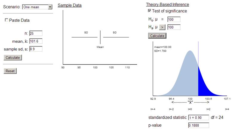
![]() = 0.90
= 0.90
e. From the graph, we can ballpark the p-value between .1 and .33 (actual value .19). Based on the t value being less than 1 and the large amount shaded on the graph, this sample mean of 101.6 is not a surprising outcome for a random sample of 25 people when the population mean equals 100.
f. If the average IQ of
this group is really 100, then we could expect to see a random sample of 25
people from this group with an average IQ of at least 101.6 in about 19% of
samples by random chance alone. As this would be a fairly common
occurrence, we have no reason to doubt that the mean IQ of the population
(those who claim to have had an intense experience with an UFO) is 100. We also
need to be willing to believe that this sample is representative of all
individuals who claim to have had such an experience.
7) a. The observational units are the adult American who
were interviewed by the GSS. The variable is the number of close friends that
the adult American has. This variable is quantitative.
b. A t-interval is valid in spite of the strong right skew because the sample size is very large (1467).
c.
95% confidence interval for ![]() , the mean number of
number friends in the population of all adult Americans: 1.987 +
2(1.7708/√1467)
, the mean number of
number friends in the population of all adult Americans: 1.987 +
2(1.7708/√1467)
= 1.987 +
.0924
= (1.894, 2.079)
Note: Theory-based
approach gives (1.896, 2.078)
We are 95% confident that the mean number of
close friends in the population of American adults is between 1.894 and 2.079
friends.
Note, if
we calculate 1.987 + 2(1.7708), we extend from below zero to about
4.4 friends. Meaning about 95% of adult
Americans report between 0 and 4.4 friends.
This is very different from the confidence interval which is a statement
about the population mean, not individual adults.
d.
The reasonable interpretations of this interval are:
- You can be 95% confident that the mean number of close
friends in the population is between the endpoints of this interval.
- If you repeatedly took random samples of 1467 people
and constructed t-intervals in this same manner, 95% of the intervals in
the long run would include the population mean number of close friends.
e. “Ninety-five
percent of all people in this sample reported a number of close friends within
this interval” is incorrect because that is not what 95% confidence refers
to (the percentage of intervals that will capture μ, not the percentage of
the sample that does something)
“If you took another sample of 1467 people, there is a 95% chance that its
sample mean would fall within this interval” is incorrect because we are
not trying to capture sample means – we are trying to capture the population
mean.
“If you repeatedly took random samples of 1467 people, this interval would
contain 95% of your sample means in the long run” is not a correct
interpretation because the interval would definitely contain the one sample mean
you used to create the interval. We cannot predict how many of the other
sample means it would contain – the interval procedure is estimating the
population mean. We are not saying other sample means should be within 2
standard deviations of the one we observed, but that sample means in general
should fall within 2 standard deviations of the actual population mean.
It
is incorrect to say “this interval captures the number of close friends for
95% of the people in the population” because this interval estimates the mean
number of friends – not the number of individual friends for any person.
f.
If the sample size were large, the interval would have the same midpoint, but
would be narrower.
If the sample mean were larger the interval would have a larger midpoint, but
would have the same width.
If the sample values were less spread out, the standard deviation would be
smaller, so the margin-of-error would be smaller, so interval would be narrower
(but would have the same midpoint).
If
every person in the sample reported one more close friend, the sample mean
would be larger (by 1), so the midpoint of the interval would increase by 1,
but the width would be
unchanged.
8) (a) The population is all American households. The sample
is the 47,000 (ish) households for which they
received a response about whether or not they included a pet cat.
(b) This tells us that the observed
sample proportion (0.324) is 4.14 standard deviations below the hypothesized
population proportion (one-third).
(c) Yes, the standardized statistic is
large (4.14 > 2) and the p-value is small (< 0.0001), so we have strong
evidence to reject the null hypothesis in favor of the alternative
hypothesis. This was presented as a
two-sided test (the not equals to in Ha), so we conclude there is evidence that
the population proportion of households that include a bit cat differs
from one-third.
(d) To answer this question, about the
size of the difference, I would look at the confidence interval rather than the
test of significance. The confidence interval (0.3198, 0.3282) is consistent
with the test in that 1/3 is not included among the plausible values. However,
they are not all that far from 1/3, telling us the percentage is around 32%
more than 33%, but that if we wanted to tell folks that the percentage is roughly
33%, we wouldn’t be considered huge liars.
This example highlights the distinction between statistical
significance (could this have happened by chance alone) and practice
significance (is it all that meaningful to you or me). Often we might need
to consult a “subject matter expert” to decide is the size of a difference is
meaningful, that’s not usually the statistician’s call.