Workshop Statistics: Discovery with Data, Second
Edition
Topic 6: Comparing Distributions I: Quantitative Variables
Activity 6-1: Birth and Death Rates
(a) See Activity 6-12
(c)
|
West
|
|
East |
| |
10 |
9 |
|
9
|
11 |
3488 |
|
9
|
12 |
358 |
|
8874430
|
13 |
01125566799 |
|
98765420
|
14 |
112 |
|
94
|
15 |
2668 |
|
331
|
16 |
|
| |
17 |
|
|
9
|
18 |
|
| |
19 |
|
| |
20 |
|
|
2
|
21 |
|
(d) The median birth rate for the eastern states is 13.5 births per 1000
residents. This median for western states is 14.45 births per 1000 residents.
(e) Answers will vary from student to student.
(f) The western states tend to have higher birth rates than eastern
states. The median is higher in the west, and the distribution of birh
rates in the west generally covers higher values than in the east.
(g) No, there are many cases where an eastern state has a higher birth
rate than a western state. One extreme example of such a pair is Georgia
and Montana.
(h) It's likely that the western state would have a higher birth rate
than the eastern state, because the distributions in the stemplot reveal
that more western states have higher values than eastern states.
Activity 6-2: Professional Golfers' Winnings
(a)
|
|
min
|
Q1
|
median
|
Q3
|
max
|
|
PGA
|
1259
|
1491
|
1675
|
2021
|
6617
|
|
LPGA
|
296
|
367
|
491.5
|
584
|
1592
|
|
Seniors
|
631
|
738
|
970
|
1118
|
2516
|
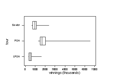
(b) Note that the tours are in a different order below:

(c) No, the boxplot would not look different because the five-number
summary would not change.
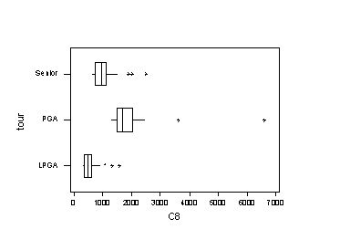
(d) LPGA: IQR = 584 367 = 217, so 1.5IQR = 325.5. Subtracting this
from the lower quartile gives 41.5. Since no woman on the list made less
than this, there are no low outliers. Adding 325.5 to the upper quartile
(584) gives 909.5. Outliers are thus Webb (1592), Inkster (1337), and Pak
(957)
Seniors: IQR = 1118 738
= 380, so 1.5IQR = 570. Subtracting this from 738 gives 168, and no senior
made less than that. Adding 570 to 1118 gives 1688, so outliers are Fleisher
(2516), Irwin (2025), and Doyle (1912).
(e) 
(f) Yes, the modified boxplots show the outliers and also how close
the non-outliers come to them (or how far they are in the PGA case!).
(g) The boxplots reveal that the PGA golfers tend to make the most,
followed in order by the Seniors and then the LPGA golfers. This difference
is exemplified by the realization that the lowest money winner among the
PGA top 30 would be a high outlier among the LPGA top 30. Also, the lowest
money winner among the Seniors' top 30 is higher than the upper quartile
among the women's top 30. The PGA winnings show the most variability (widest
box). All three distributions of earnings are skewed to the right (lower
quartile is closer to median than upper quartile).
Click here
to see answers for (f)-(i) in Minitab version.
Activity 6-3: Variables of State (cont.)
Region 1 is the West, 2 is the Northeast, 3 is the Midwest, and 4 is the
South. Some clues are the high rates of college graduates and single persons
in region 2 (Northeast), the high rate of teen mothers in region 4 (South),
and the high rate of people of Mexican descent in region 1 (West).
Activity 6-4: Top American Films
(a)
|
|
number
|
mean
|
std. dev.
|
min
|
Q1
|
median
|
Q3
|
max
|
|
won Oscar
|
32
|
34.13
|
18.23
|
6
|
22.25
|
33
|
46.75
|
70
|
|
did not
|
68
|
43.56
|
17.99
|
4
|
30.25
|
44.5
|
59.75
|
85
|
(b) 
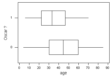
Both distributions look fairly symmetric with maybe a slight skew to
the right for movies that did won the Oscar (1's). The movies that won
an Oscar tend to have lower age values than moves that did not win the
Oscar. Both distributions show a large spread with slightly more variability
among the ages of movies that did not win the Oscar.
(c)-(e) Answers vary from student to student.
