Workshop Statistics: Discovery with Data, Second
Edition
Topic 17: Sampling Distributions II: Means
Activity 17-1: Coin Ages (cont.)
Click here
for answers for Minitab version.
(a) observational units: pennies; variable: age, quantitative
(b) parameters; mean: m; standard
deviation: s
(c) No, this distribution is skewed to the right.
Students' answers to (d)-(l) may differ since
the data are chosen randomly. These are meant to be sample answers.
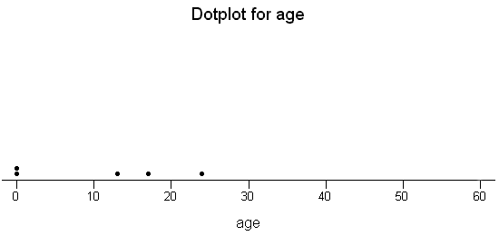
(d) 13, 24, 17, 0, 0

(e) 10.8
(f)
|
Sample no.
|
1
|
2
|
3
|
4
|
5
|
|
Sample mean
|
10.8
|
13
|
5.8
|
12.8
|
17.8
|
(g) No, this is an example of sampling variability. This is a quantitative
variable, rather than a categorical one.
(h) mean of  values: 12.04; standard deviation of x-bar values: 4.33
(i) This mean is reasonably close to the population mean. This
standard deviation is less than the population standard deviation.
(j)
(k) This distribution appears to centered near the population mean
of 12.264. The values are less spread out than the population distribution
and the five sample means of size 5.
(l) yes
Activity 17-2: Coin Ages (cont.)
Students' answers to (a)-(m) may differ since
the data is chosen randomly. These are meant to be sample answers.
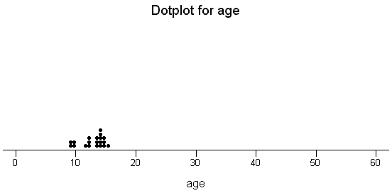
(a)
Yes, it resembles the distribution
of ages in the population.
(b) mean: 12.8; standard deviation: 9.228; Yes, they are
reasonably close to their population counterparts. The distribution
is skewed to the right.
(c)
This distribution does not
have as wide a spread. The shape is much less skewed.
(d) mean: 12.426; standard deviation: 4.072; The mean is
pretty close, but the standard deviation is lower.
(e)
The spread is even more
narrow and mound shaped now, as variability decreases.
(f) mean: 12.098; standard deviation: 1.715; The mean is
still close, but the standard deviation is even lower now.
(g)
Again, the distribution
narrows and the variability decreases. The distribution has become
more normal.
(h) mean: 12.02; standard deviation: 1.371; The mean is
still close, but the standard deviation is slightly lower than before.
(i) Although answers may vary, the correct answer is yes.
(j)
This distribution is roughly
normal.
(k), (l, k)
| |
Mean
|
Std. dev.
|
Shape
|
|
Population 1
|
m = .5
|
s= .289
|
uniform
|
|
Sample Means of size n = 50 from 1
|
.49937
|
.03637
|
|
|
Population 2
|
m = .5
|
s = .354
|
u-shaped
|
|
Sample means of size n = 50 from 2
|
.50264
|
.04686
|
|
(l)
This distribution is roughly normal.
(m) Penny ages: 1.359; 1: .041; 2: .050
Activity 17-3: Christmas Shopping
(a) It is a statistic because the 922 adults are meant as a sample
of the population of all American adults who plan to buy Christmas gifts
that year.
(b)
-
population of interest: American adults who expected to buy Christmas gifts
in 1999
-
sample selected: 922 American adults polled on November 18-21
-
parameter of interest: money expected (mean amount) to be spent on Christmas
gifts
-
statistic calculated: sample mean was $857
(c) m is not necessarily equal to $857, though
it is possible. All values listed for are m possible,
with the different sample mean arising by chance alone.
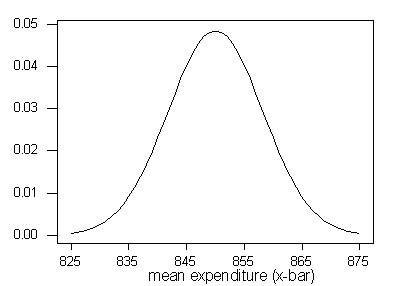
(d) The central limit theorem says that the sample means would vary
like a normal distribution with mean $850 and standard deviation 250/sqrt(922)=8.23
if samples of size n = 922 were taken over and over. This
does not depend on the shape of the distribution of expected expenditures
in the population since the sample size is large.
(e)

(f) No, since this is a normal distribution, $857 is near the center
of the distribution, well within one standard deviation of the mean.
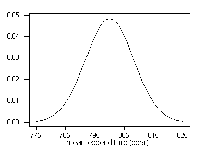
(g, d) The sample mean would vary over a normal distribution with mean
$800 and standard deviation 8.23 if samples of size n = 922 were
taken over and over.
(g, e) The picture would be the same, just shifted to center around
800:

(g, f) Now $857 is way in the tail of the distribution. This would
be a very unlikely sample mean if the population mean was equal to $800.
(h) The CLT says that the standard deviation of the sampling distribution
of the sample mean should be 250/sqrt(922) = 8.23.
(i)2(8.23)=16.46
857-16.46=840.5
857+16.46 = 873.46
interval for m: ($840.54, $873.46)


