Stat 301 - HW 4

Due noon Friday, Feb. 7

You can bring a hard copy to class Thursday, to my office Friday, or upload in Canvas by noon Friday. No late assignments will be accepted. If electronic, remember to upload separate files for each problem and to put your name inside each file. All computer output should be integrated into the body of your write up. Your computer output and writeup should be done individually. Remember to show your work/calculations/computer details.

To open the data files (See p. 33 of the text)

In R

· You can follow the link and copy and paste all of the data to the clipboard (e.g., ctrl-A, ctrl-C). Then in R you can type

PC: > AnthemTimes = read.table("clipboard", header = T)

MAC: > AnthemTimes = read.table(pipe("pbpaste"),header=TRUE)

· You can download and save the file and then use Import > Dataset

In JMP

· You can follow the link and copy and paste all of the data to the clipboard (e.g., ctrl-A, ctrl-C). Then in JMP, open a new Data Table (e.g., File > New) and then select Edit > Paste with Column Names

· You can download and save the file and then use Files > Open and then choose the file type

1) So we collected data on the length of the performance of the national anthem preceding the National Football League’s Super Bowl for games from 1980 (Super Bowl 14) to 2019 (Super Bowl 53). AnthemTimes.txt

(a) What are the observational units? What are the variables? Which variables are quantitative and which are categorical? For quantitative variables, what are the measurement units? For categorical variables, what are the categories?

(b) Create a dotplot of the anthem times (see p. 134. In JMP, can also follow the link in the journal file). Give a brief description of the distribution, as if to someone who can’t see it. Also report the mean and standard deviation, and the five-number summary (p. 137).

(c) Identify the outliers in the distribution by name. Test whether these observations are outliers according to the “1.5IQR” criterion (p. 142).

(d) Create a normal probability plot for these data (p. 144). Would you consider the normal distribution to be a good model for these data? Explain your reasoning.

(e) Split the dotplot by Sex. Compare the two distributions.

In R: iscamdotplot(Time, Sex) and iscamsummary(Time, Sex)

(f) Split the dotplot by Genre2. Compare the distributions.

2) I downloaded a random sample of 2,000 responses to the 2017 American Community Survey (https://www.census.gov/programs-surveys/acs). The variable income-wages reports each respondent’s pre-tax wage or salary income received for work performed as an employee. Amounts are expressed in 2017 dollars. IncomeWages2000.txt or IncomeWages2000.csv

(a) Create a graph of income-wages. Is there an explanation for the 999999 values? Should they be removed from the dataset? (Document any detective work you use.)

(b) Subset the data (p. 134), removing those under the age of 18 and those with N/A for weeks worked. Recreate a graph of income-wages. Describe the shape of the distribution and what it represents in this context.

(c) Report the values for the mean and the median. How do they compare? Is this what you would have expected based on the shape? Which would you report as a “typical” wage? Explain.

(d) Determine the median wage for women and median wage for men in 2017. Examine the ratio-how much do women make for every $1 men make, “on average.”

(e) Examine the graph below showing how the mean and median wages have changed over time.

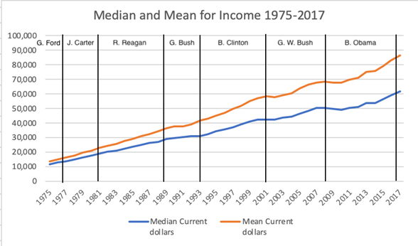
Comment on what this tells you about “income inequality” in the United States.

3) Open the Sampling from a Finite Population applet. The default population represents the sleep times (hours slept the previous night) of 18,000 students.

(a) Make a screen capture of the population distribution. Summarize the shape, center, and variability. What symbols would you use to refer to the mean and to the standard deviation?

(b) Check Show Sampling Options and use the applet to draw 1,000 samples of 10 students from this population. Check the Overlay Normal Distribution box. Include a screen capture of the distribution of sample means. Report the mean and standard deviation of the distribution of sample means. Note: I wouldn’t try to take more than 1,000 samples with this applet.

This assumes the population distribution of sleep times is skewed to the right, but with a population mean again around 8 hours and a standard deviation again around 1.5 hours. If we were to take 1,000 samples of 10 students from this population, do you expect the distribution of sample means to be approximately normal? What do you/the Central Limit Theorem for sample means predict for the mean and standard deviation of the distribution of sample means (p. 152)?

(d) Generate the 1,000 samples and verify/change your predictions from (c). Overlay the Normal Distribution and count how many sample means are 7.25 or less. [Include a screen capture.] Are the simulation results and the normal probability results similar? Is it surprising to find a sample mean of 7.25 hours or less in a sample of 10 students from population 2?

(e) Now change the sample size from n = 10 to n = 50. What do you/the Central Limit Theorem for sample means predict for the shape, mean, and standard deviation of the distribution of sample means (p. 152)?

(f) Generate the 1,000 samples and verify/change your predictions from (e). Overlay the Normal Distribution and count how many sample means are 7.25 or less. [Include a screen capture.] Are the simulation results and the normal probability results similar? Is it surprising to find a sample mean of 7.25 hours or less in a sample of 50 students from population 2? More or less surprising than with a sample size of 10 students?

(g) Calculate a z-statistic to measure the distance between a sample mean of 7.25 hours and a population mean of 8 hours, assuming a population standard deviation of 1.5 hours and a sample size of 50 students.

(h) Now consider a sample of 1,000 people from this population. What does the Central Limit Theorem predict for the standard deviation? Take 1,000 random samples in the applet, what is the standard deviation of the 1,000 sample means? How does this compare?

What if you apply the finite population correction factor ? (p. 109)

(i) Choose the Gettysburg population.

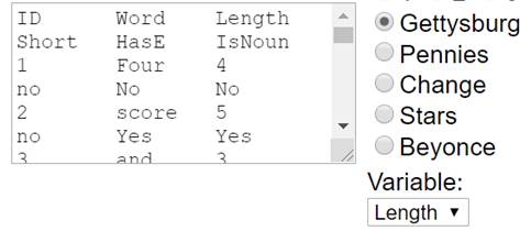
Using the length variable, describe the shape, mean, and standard deviation of the population.

(j) Generate a sampling distribution of 1,000 sample means of size 20 for the length variable. What is the standard deviation? (Include a screen capture)

(k) Check the Stratify Samples by box and select Short. Select one random sample of 20 words. How many are short and how many are long? Select another random sample of 20 words, how many are short and how many are long?

(l) Generate a sampling distribution of sample means using stratified sampling (include a screen capture). How does the standard deviation compare to (j)? Why?

Possible Extensions Assignments

· Add to our National Anthem dataset. Discuss another interesting bet you could make in the Super Bowl.

· Critique/Comment on the use of statistics during the Super Bowl broadcast. What was the best use of statistics? What was the worst?

· Find a recent article on income inequality or the gender gap and compare the discussion to the data in problem 2. (e.g., Elizabeth Warren speech https://www.youtube.com/watch?v=7LNyuKwORV4)

· Learn about the Gini index and how it is calculated and how it measures income inequality.

· Check out the World Income Inequality database, produce a graph for the USA over time and comment on what it reveals.

· Find an article that uses stratified sampling. Why did they do so? Did it appear to be effective?

· Carry out the simulations in problem 3 in R. Document your exploration.

· Work though Introductions to Databases and/or Introduction to Querying at the Databases for Many Majors website. Summarize what you learn.