INVESTIGATING STATISTICAL CONCEPTS, APPLICATIONS, AND METHODS
NOTES FOR INSTRUCTORS
Chapter 1 Chapter 2 Chapter 3 Chapter 4 Chapter 5 Chapter 6
General Notes:
We envision the materials as being very flexible in how they
are used. You may choose to lead
students through many of the investigations together as a class, but we also
encourage you to give students time to work through some questions on their own
(or better in pairs) and then debrief with the students afterwards. If
you do have students work through investigations largely on their own, it’s
very important to conduct a wrap-up discussion at the end of class, and/or at
the beginning of the next class, in which you make clear what the “morals” of
the investigations were. In other words, summarize for students what they
were supposed to have learned through the investigations and what they are
responsible for knowing, making sure they are reading the additional exposition
in the text as well. These wrap-up discussion times are also ideal for
inviting students’ questions, because they will have wrestled with the ideas
enough to know what the issues are and where their understanding is shaky. You may wish to collect students’
answers to just a few of the questions in an investigation to read over and
give feedback before the next class session.
The practice problems are intended to provide students with basic review
and practice of the most recent ideas between class periods. This will help structure their time outside
of class, and provide a way for you and the students to informally assess their
understanding and provide feedback. You
may choose to collect and grade these as homework problems or use them more to
motivate initial discussion in the next class period. You can also consider including a “participation”
component in your syllabus to include effort if your evaluation will be more
informal. Solutions have been posted
online. They are password protected
giving the instructor the option of giving students direct access or not. These problems also work well in a course
management system such as Blackboard or WebCT for
more automatic submission and feedback.
You may also wish to supplement some of the material in the book, e.g., bringing in recent news articles for discussion, assigning data collection project assignments. We think students will find these investigations interesting and motivating, but there will also be time to share other examples as well. You may also wish to have students refer to the additional examples we have posted here. If you do bring in your own material, we do caution you to try to remain consistent with the text in terminology, notation, and sequencing of ideas. Some of this may be different for you as the instructor and may take a while to get used to. Keep in mind that the material you think is usually introduced at different points in the course will be coming eventually.
We have written the materials assuming students will have easy access to a computer, and we make increasing use of technology as the course progresses. We have taught the course with daily access to a computer lab, but believe it will also work with less frequent visits to a computer lab and/or more instructor demonstrations (using a computer project system). If the students do not have frequent access to computers during class, you may wish to assign more of the computer work to take place outside of class. We do provide detailed instructions for all of the computer work (Minitab, Excel, java applets), but you may still want to encourage students to work together. We have also assumed use of Minitab 14 but at the Minitab Hints page will try to outline where you will have to make adjustments to use Minitab 13. Even with heavy use of computers, it is also nice to have some days where you focus less on the computers to give students a chance to ask questions on the larger concepts in the material and even work a few calculations “by hand.” Student will use a calculator on a daily basis as well.
You might consider giving an exam after Chapter 2 and then either after Chapter 4 or 5 depending on how deep you will be able to go into the chapters.
Section 1-1:
Summarizing Categorical Data
Timing: Taking roll, explaining the syllabus, telling them a bit about what the course would be like, and then going through most of the section together took about 60 minutes. Students are asked to make a graph in Excel but that can be easily moved to outside of class (perhaps after an instructor demonstration).
Some additional information about the study in Investigation 1-1:
- Appeared in August, 2002 New
- You can also find some links on the web to the ensuing court case. A recent one may still be here or here.
- In May, 2000: eight persons who had worked at the same microwave-popcorn production plant were reported to have bronchiolitis obliterans. No recognized case was identified in the plant. Therefore, they medically evaluated current employees and assessed their occupational exposure in Nov. 2000.
- They used a combination of questionnaires and spirometric testing. They also compared information to the National Health NE Survey
- The results here focus on the results of the spirometric testing: 31 people had abnormal results, 10 with low FVC (forced vital capacity) values, 11 with airway obstruction, and 10 with both airway obstruction and low FVC.
- Diacetyl is the predominant ketone in artificial butter flavoring and was used as a marker of organic-chemic exposure
- They tested air samples and dust samples from various areas in the plant. These areas included
Plain-popcorn packaging line, bag-printing areas, warehouse, offices, outside
Quality control or maintenance
Microwave-popcorn packaging lines
Mixing room
The first group is considered “non-production” so lower exposure but they also looked at how long employees had worked in different areas to classify them as “high exposure” and “low exposure.”
In (e), get students to tell you about their description of the graph – solicit descriptions from several people. Make sure the descriptions are in context and include the comparison, but then you will probably be able to tell them that all the responses were good and that’s one distinction between statistics and other subjects, that there can be multiple correct answers. When students offer suggestions about reasons for the difference in the groups, make sure they discuss a factor that differs between the two groups. So saying “other health issues” isn’t enough, but saying that those who worked in certain areas of the plant may have different SES status than those who work in the production areas of the plant or that they may be more likely to live in the country which has different air quality, etc. Really get them to suggest the need for comparison, either to people outside the plant or to people in different areas of the plant. Also build up the idea of not just comparing the counts but converting to proportions first.
In (k), we encourage you to go through the odds ratio calculations especially. You might consider asking a student in the class to define odds, but you need to build up the odds ratio slowly and always encourage them to interpret the calculation correctly.
Page 7: It’s important that students get a chance to practice with the vocabulary soon as it is not as easily mastered as they may initially think. You especially need to watch that they state variables as variables. Too often they will want to say “lung cancer” instead of describing the entire variable. Or they will slip into summaries like “the number with lung cancer.” Or they will combine the variables and the observational units: “those with lung cancer.” We strongly recommend trying to get them to think of the variable as the question asked of each observational unit.
The practice problems are intended to get students to work more with variables and to make sure they can do the two-way table and segmented bar graphs. Much of the terminology will be unfamiliar to them or they will have other “day-to-day” definitions so it is important to “immerse” them into the vocabulary and allow them to practice it often. We suggest beginning the next class by discussing these problems, especially 1-1f and 1-2. Problem 1-3e is an important issue that may or may not come up in your initial class discussion but not everyone given the survey filled it out. You need to worry about the people who may have been home sick or even the people who became so sick they no longer work at this factory. We highly encourage you to either collect students’ work on the practice problems (reading through and commenting on their responses) and/or to briefly discuss them at the beginning of the next class period. We envision these as being a more informal, though provoking, self-check form of assessment.
We have included “section summaries” at the end of the sections in Chapter 1. This is a good place to ask students if they have questions on the material so far. You might also consider adapting these into bullet points to recap the previous class period at the start of the next class period. You may want to remind students occasionally that they should read all of the study conclusion, discussion, and summary sections carefully; some students get in the habit of working through the investigations by answering questions but do not “slow down” enough to read through and understand the accompanying exposition.
Section 1-2: Analyzing Categorical Data
Timing: Students were able to complete this section in approximately 90 minutes. You may wish to have students complete some of the Excel work outside of class (including for Investigation 1-2 prior to coming to class). We did Investigation 1-2 mostly together but then students worked on Investigation 1-3 in pairs. There is an Excel Exploration but no other technology is used.
Investigation 1-2 gives students immediate practice in applying the terms. We strongly encourage you to allow the students to work through these questions, at least through (j), on their own first. Question (c) asks students to use Excel, but again they could do that outside of class or you could demonstrate it for them. Students will struggle and you need to visit them often to make sure they are getting the answers correct (e.g., how they state the variables, whether they see “amount of smoking” as categorical, and calculation of the odds-ratios). The odds-ratios questions are asked to encourage them to treat having lung cancer as a success and putting the non-smokers odds in the denominator. This ensures the odds-ratio is greater than one and treats the non-smokers as the reference group to compare to. (Though students may have some trouble getting used to treating having lung cancer as a success!) The main criticism we expect to hear about in (j) is age but even after the odds-ratios were “adjusted” for age there could be other differences between the groups again, e.g., socio-economic status, diet, exercise that is related to both smoking status and occurrence of lung cancer. Don’t expect perfect answers on (j) and (k) but give them a chance to think about the issues before you discuss them together. Question (l) contains a typo; the question should be about “lung cancer patients” not “smokers” (you can joke that it certainly doesn’t tell us about the proportion of smokers, but also not about lung cancer patients in general). This is a subtle point but important for students to think about. You should give students a chance to think about the issue for a while before you discuss it with them.
In this text, we tend to distinguish between the types of study (case-control, cohort, cross-classification) and the type of design (retrospective, prospective). These are not clear distinctions and you may not wish to spend too long on them (the definition of a cohort study given is especially simplistic). Mostly you will want students to distinguish between observational studies and experiments, but also always considering the implications of the study design on the final interpretations of the results. You can ask them to read the discussion on p. 15 outside of class. One note on how we use the “definition” boxes. The top of the box is generally a generic definition. The bottom of the box will be how the term applies in the particular study being discussed.
Questions (m) and (n), about when we can draw cause/effect conclusions and when we can generalize results to larger population, are important ones that will arise throughout the course, so it’s worth drawing students’ attention to them. In particular, we want students to get into the habit of seeing these as two distinct questions, answered based on different criterion, to always be asked when summarizing the conclusions of a study. Students probably won’t have great intuition here so give them time to struggle with these questions first, without expecting perfect answers, then discuss them together. These points will come up repeatedly throughout the course. In the following discussion, we touch on the debate of whether “lung cancer” should be considered a variable. We tend to fall in the camp that it is a variable but students need to be clear that that fact that the distribution of the variable was controlled by the researchers affects the types of conclusions we can draw.
Questions (o)-(t) are good ones to discuss as a class (note the typo in the ordering of r-s). You should remind students that you have shifted gears here a bit and are now looking at properties of these calculations. You might consider dividing up the calculations in (o)-(s), assigning different groups of students to work on each question and share their results with the class. These questions are a good example of where even good students might answer the questions well but miss the point behind the calculations, so you might want to hold a follow-up discussion or at least draw students’ attention to the discussion section in the book. Students should be able to tell you that it doesn’t make sense to calculate the proportions conditional on the smoking level since the lung cancer “variable” was controlled by the researchers. This is a subtle point that you may not want to belabor but it begins to explain to students why we use the odds ratio in many situations instead of the more easy to interpret relative risk. Similarly, the “invariance” of the odds ratio to how we define success and failure is another advantage.
Investigation 1-3 provides students with more practice and gets them to again think in terms of association. They should be able to tell you some advantages to the prospective design over the retrospective design (e.g., not relying on memory, seeing what develops instead of taking people who are already sick). However this does not take into account any of the other possible confounding variables or that they only selected healthy, white men initially. You may want to pre-create the Excel worksheet for them and then have them open it and start from there.
The Excel Exploration can be done inside or outside of class. I had students finish it in pairs outside of class and then turn in a report of their results. They should see that the odds-ratio and the relative risk are similar when the baseline risk is small and that they can be very different from 1 even for the same difference in proportions. This is also the first time they really see that the OR and RR are equal to one when the difference in proportions is zero. We encourage you to have them view the updating bar graph throughout these calculations to also see the changes visually. This exploration is essentially playing with formulas but allows them to come to a deeper understanding of the formulas, how to express them, and hopefully how they are related. Some issues you might want to ask them about afterwards (in class or in a written report) include:
- when will RR and OR be close together (you can even lead a discussion of the mathematical relationship OR = RR(1-p2)/(1-p1) )
- when are RR and OR more useful values to look at than the difference in proportions (primarily when the success proportions are very small or very large)
- when will RR and OR be equal to 1 and what does that imply about the relationship between the variables/the difference in proportions
These comparisons should fall out if they follow the structure of the examples and what changed with each table. The last questions in (l) also try to help them distinguish between saying the probability of success is the same across groups and the probability of success is the same as the probability of failure. They should realize that the latter condition is not required for independence. Part (m) is where we try to direct their summary of the issues, you may wish to add even more structure there. A 5-point scale appeared to work well in grading this paragraph. You also need to decide how much of the Excel output you want them to turn in.
As you summarize these first 3 investigations you might even
want to warn them that they won't see RR and OR too much for a while but the
other big lessons they should be taking from this early material is the
importance of the study design and always using graphical and numerical
summaries as they explore the data. Students should also be getting the idea
that statistics matters and that statistics is important for investigating
important issues.
Additionally you can highlight the three studies they have
seen so far (Popcorn, Wynder and Graham,
|
Popcorn and lung disease |
Wynder and Graham |
|
|
Defined subjects as high/low exposure, classified airway obstruction |
Found subjects with and without lung cancer, classified smoking status (case-control, retrospective) |
Found level of smoking, followed subjects, whether died of lung cancer (cohort, prospective) |
|
Meaningful to examine proportion with airway obstruction |
Not meaningful to examine proportion with lung cancer |
Meaningful to examine proportion who died of lung cancer and proportion of smokers |
|
Similar number in each explanatory variable group |
Similar number in each response variable group |
|
|
May not be representative |
Controlled interviewer behavior |
Not much control (22,000 ACS volunteers) |
Section 1-3
Timing: This section will probably take approximately 45-50 minutes. You may choose to do more leading in this section in the interest of time. No technology is used.
The initial steps of Investigation 1-4 should be fairly routine for students by this point. You might consider asking them to complete up to a certain question before they come to class. It is also fun to ask them whether or not they wear glasses and if they remember the type of lighting they had as a child. The key point is of course the distinction between association and causation and through class discussion students should be able to suggest some reasonable confounding variables. Where to be picky is to make sure that their confounding variable has a clear connection to the response (eye condition) and that there is the differentiation in this variable between the explanatory variable groups (type of lighting). You might consider having them practice drawing an experimental design schematic (formally introduced later in the course), along with matching the different confounding variable outcomes with the different explanatory variable outcomes. For example:
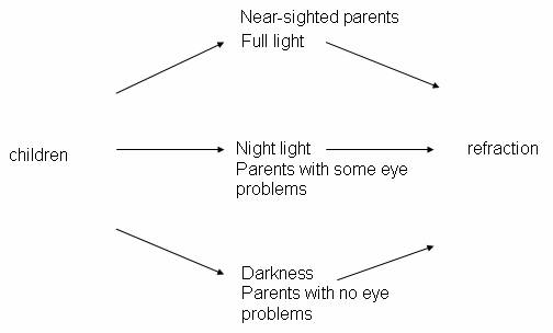
The practice problems at the end of this investigation are a little more subtle and it will be important to discuss them in class and ensure that students understand the two things they need to discuss to identify a variable as potentially confounding (its connection to both the explanatory and the response variable).
In Investigation 1-5, we have chosen to treat Simpson’s Paradox as another confounding variable situation. This investigation goes into the mathematical formula as another way to illustrate the source of the paradox (the imbalance in where the women applied and an imbalance in the acceptance rates of the two programs). You might also consider showing them a visual illustration such as:
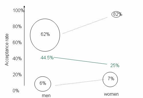
where the size of the circles are intended to convey the sample sizes in each category and thus their “weight” in the overall calculation.
There is a typo in questions (i) and (k), they should ask whether the overall acceptance rate for women is equal to the average of the acceptance rates in each program, not about Simpson’s Paradox. This change greatly simplifies the questions and students should not have much trouble. However, then this is purely about weighted averages and not Simpson’s Paradox. If you really want to challenge the students, you can ask them to work with the weighted averages to derive mathematically (or at least verify) conditions where Simpson’s Paradox will not occur. Click here for an example discussion, which could also be turned into a homework problem.
The practice problems will help them see the paradox arising in different settings. Even when they see and pretty much understand what’s going on, students often struggle to provide a complete explanation of the cause of the apparent paradox. A very good follow-up question is to ask them to construct hypothetical data for which Simpson’s Paradox occurs as in the following homework problem: Suppose two softball players each have 200 at-bats over 2 months in the season. Construct a two-way table so one player has a higher average (success proportion) for each month individually, but the other player has a higher average (success proportion) over these 200 at-bats.
It will be important to convey to students exactly what “skills” and “concepts” you want them to take away from this investigation. If you want to focus on the “weighted average” idea (which has some nice reoccurrences later in the course), students will probably need a bit more practice. In summarizing these investigations with students, we are hoping they have motivated the need for more careful types of study designs that would avoid the confounding issues. Students often have an intuitive understanding of “random assignment” but this will be developed more formally in the next section.
Section 1-4: Designing Experiments
Timing/Materials: This section will probably take approximately 45-50 minutes and consists of several small investigations. Try to focus on the big issues tying the investigations together. Some of the simulations could be assigned to out of class. You will need index cards for the tactile simulation and access to an internet browser. You should get the students in the habit of going to the main data files and java applets page here and selecting from that page.
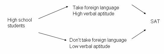
In Investigation 1-6, students see yet another example of the limitations of an observational study and are usually very good at identifying potential confounding variables. It’s fun to ask students if they know whether their institution has a foreign language requirement and what might be the reasons for that requirement. Deciding whether foreign language study directly increases verbal ability (as posited by many deans), this leads into the idea of an experiment and most students appear to have heard these terms, including placebo, before. We would recommend going through this investigation with the students rather quickly. A schematic on p. 37 is missing:
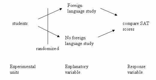
You may also wish to
discuss with them the schematic for the original observational study and the
potential “verbal ability” confounding variable:
In Investigation 1-7, we strive to help students see the need for randomization. We have students begin with a hands-on simulation of the randomization process. We feel this engages the students and gives them a concrete model of the process. We encourage you to have the students come to the board to collectively create the dotplot of their results in (d). Students could conduct the randomization outside of class and bring in their results but we feel this concept is important enough that you may prefer to do so in class. Students then transition to an applet to perform the randomization process many, many more times. Hopefully the prior hands-on simulation and the graphics of the applet will help them connect to the computer simulation (and reinforce that they are mimicking the randomization process used by the researchers). They should be able to work through the applet questions fairly quickly and then you will want to emphasize that randomization “evens out” other lurking or extraneous variables between the groups. It is important to emphasize to students that while we often throw around the word “random” in everyday usage, achieving true “statistical randomness” takes some effort and should not be short-circuited.
Investigation 1-8 is listed as optional or may be presented briefly. It continues to use the applet to have students think about the concept of “blocking.” We have chosen to discuss a rather informal use of “blocking” in that students are grouping subjects into homogenous units. [A more formal introduction to blocking would only allow the block size to equal the number of treatments.] Students can again play with the tactile simulation or you can consider question (b) as a “thought experiment” since they should see the effect pretty quickly. The applet conveys the idea that if you actively balance out factors such as gender between the two groups, that will ensure further balance between the groups on some other variables as well (those related to gender, like height). We chose not to emphasize this concept strongly but did want students to think about the advantages (and disadvantages) of carrying out the experimental design on a more homogeneous group of subjects.
At this point in the course, you might also consider assigning a data collection project where students work with categorical variables and consider both observational and experimental studies. An example assignment is posted here.
Section 1-5: Assessing Statistical Significance
Timing/Materials: With some review of the idea of confounding variables at the beginning, this section takes approximately 60 minutes. One timing consideration is in having students do a second tactile simulation. This simulation is very similar to that in Section 1-4 but here focuses on the response instead of the explanatory variable. Still, you may want to make sure these simulations occur on different days. We do see value in having them do both as students too easily forget what the randomization in the process is all about. This simulation also ties closely to an applet and helps transition students to the concept of a p-value. You will need pre-sorted playing cards or index cards and access to an internet browser. We pre-sort the playing cards into packets of 24, with 11 red ones (hearts/diamonds) representing successes and 13 black ones (clubs/spades) representing failures, but you could also use index cards and have students mark the successes and failures themselves.
The goal in this section is to see the entire statistical process, from consideration of study design, to numerical and graphical summaries, to statistical inference. Students learn about the idea of a p-value by simulating a randomization test. While in the previous section we focused on how randomization evens out the effects of other extraneous variables, here the focus is on how large the difference in the response variable might be just due to chance alone. You will want to greatly emphasize the question of how to determine whether a difference is “statistically significant.” Try to draw students to think about “what would happen by chance,” even before the simulation, as a way to answer this question (around question (f)). At some point (beginning of class, around question (f), end of class) you may even want to detour to another example to illustrate the logical thinking of statistical significance. One demonstration that we have found effective is to have a student volunteer roll a pair of dice that look normal but are actually rigged to roll only sums of seven and eleven (e.g., unclesgames.com, other sources). Students realize after a few rolls that the outcomes are too surprising to have happened by chance alone for normal dice and thus provide compelling evidence that there is something fishy about the dice. It is important for students to think of the randomization distribution as a “what if” exploration to help them analyze the experimental results actually obtained.
For part (i) of Investigation 1-9, we have students create a dotplot on the board, with each student placing five dots (one for each repetition of the randomization process) on the plot. You can also have students turn in their results for you to compile between classes or have them list their results to you orally (or as you walk around the room) while you (or a student assistant) type them into Minitab or place them on the board yourself.
The data described in Investigation 1-9 have been slightly altered. In the actual study, 11 observers were assigned to Group A and 12 to Group B, however we preferred that these column totals were not the same as the row totals. Students should find the initial questions very straight forward and again you could ask them to complete some of this background work prior to the class meeting. Some notes on the applet:
- holding the mouse over the deck of cards reveals the composition of the deck (students should note the 13 red and the 11 black cards).
- the alignment of the tick marks and the horizontal scale tends to be better in Netscape than in Internet Explorer.
- with 1000 repetitions, when you “show tallies” the values tend to crash a bit, but students should be able to parse them out.
- the “Difference in Proportion” button is to help students
see the transition between this distribution and the distribution of ![]() A –
A – ![]() B that
they will work with later but it may not be worth addressing at this point in
the course.
B that
they will work with later but it may not be worth addressing at this point in
the course.
- we encourage you to continually refer to the visual image of the empirical randomization distribution given by the applet when interpreting p-values.
There are some important points for students to be comfortable with in the discussion on p. 54. In particular, how the p-value presents a measure of the strength of evidence along a continuous scale. You will also want to emphasis that the p-value measures how often research results at least this extreme would occur by chance if there was no true difference between the experimental groups. You might also want to remind students that the terminology introduced in this investigation will be used throughout the rest of the course.
Brief Introduction to Minitab
You may wish to initially demo Minitab to your students while going over some of these basic features and then requiring students to open Minitab outside of class and mimic the steps you have shown them. From this point out in the course, Minitab will be used rather heavily.
Section 1-6: Probability and Counting Methods
Timing: This section, consisting of two investigations, should take approximately 45 minutes. You may also choose to supplement with some other probability applications and/or discussion of lotteries. Minitab is used in both investigations.
At this point, quantitatively inclined students are often chomping at the bit for a more analytic approach to determining p-values that circumvents the need for the simulations. Investigation 1-10 introduces them to the idea of probability as the long-run relative frequency of an outcome. Minitab is used to carry out a simulation (cast as a randomization to address statistical significance, to parallel the earlier investigations) and then graph the behavior of the empirical probability over the number of repetitions. This is the first time students create and use a Minitab macro. We initially have them copy and paste session commands to reinforce the repetition (Note: while copying and pasting the commands in the Session window is often much quicker, many students tend to prefer using the menus). After doing this for a while, students are often ready to create a program that repeats these commands for them a large number of times. Some students will pick up these programming ideas very quickly, others will need a fair bit of help. You may want to pause a fair bit to make sure they understand what is going on in Minitab. If a majority of your students do not have programming background, you may want to conduct a demonstration of the procedure first. The two big issues are usually helping students save the file in a form that is easily retrieved later and getting them into the habit of using (and initializing!) a counter. We suggest using a text editor rather than a word processing program for creating these macro files so Minitab has less trouble with them. In saving these files, you will want to put double quotes around the file name. This prevents the text editor from adding “.txt” to the file name. The macro will still run perfectly fine with this extension but it is a little harder for Minitab to find the file (it only automatically lists those files that have the .mtb extension – you will need to type *.txt in the File name box first to be able to see and select the file). On some computer systems, you also have to be rather careful in which directories you save the file. You might want students to get into the habit of saving their files onto floppies or onto the computer desktop for easier retrieval. These steps may require some trial and error to smooth out the kinks.
There is a large typo on p. 60 – the Discussion and confidence interval should not be there but rather the page should start with question (i).
The graph created on p. 61 is worth seeing as it shows the relative frequency as a function of the number of repetitions. Having students type in these commands is rather mechanical but we think it is important for them to create the graph with their own data instead of merely being shown a static picture. Still, it will be important to have longer discussions on what the pictures represent (either as a class or a writing assignment). The key will be in not letting the computer work overwhelm the larger concepts here.
This is also the first point in the course where we require students to make predictions. It’s important for students to know that this is informal and that you are only interested in their first thoughts, they should not worry about correctness at this point. We employ this strategy a lot to get students to take a stake. If their prediction is incorrect, then they are more likely to take the time to correct their misconception.
At this point you may choose to introduce some other interpretations of probability, e.g., subjective probability, to introduce them to the diversity of uses of the term. Also, while the calculations in this course often make use of the equal probability of outcomes from the randomization, you might want to caution them to not always assume outcomes are equally likely. The following transcript from a Nightline broadcast a few years about may help bring home the point:
TED KOPPEL: Dr. Andrews, I'm sure you have heard such cautionary
advice before so on what basis is the assumption being made that this is the
one that's going to have the kind of impact on southern California in
particular that's being predicted?
RICHARD ANDREWS: Well, in the business that I'm in and that local
government and state government is in, which is to protect lives and property,
we have to take these forecasts very seriously. We have a lot of forecasts
about natural hazards in
In Investigation 1-11, students use this basic probability knowledge to derive the formula for the hypergeometric probability. We hope students will become comfortable using Minitab to calculate these probabilities and try not to spend too long on the combinations calculations. You can also use Minitab or other software to show them lots of graphs of the hypergeometric distribution for different parameter values. Make sure on p. 67 they see the subcommand at the top of column 2. Students will vary in their comfort levels with the binomial coefficient and calculations. You may wish to help students maintain focus on the “end result” and make more use of technology to calculate the probabilities (including showing your students how to do these combination calculations on their calculator). We often also advise them that we are more interested in their ability to set up the calculation (e.g., on an exam) and to interpret the result (and make decisions based on the value). You should consider helping students see in the pattern in the hypergeometric combinations with the top numbers in the numerator adding to the top number in the denominator and the bottom numbers adding as well. We also help to help student continue to distinguish between “empirical” and “theoretical” probabilities, and we strive to keep the “statistical motivation” of these calculations in mind – how often do experimental results as extreme as this happen “by chance.”
The Random Babies applet in Practice 1-20 is fun and often memorable for students. While the applet repeats the concepts of the Minitab simulation it may be more visually appealing for students. You may want to apologize about the possibly offensive context ahead of time.
Section 1-7: Fisher’s
Exact Test
Timing: This section, along with Chapter 1 review, should take about 50 minutes. You may also wish to provide more practice carrying out Fisher’s Exact Test and discussing the overall statistical process. In the Investigation, students are asked to create a segmented bar graph and calculate p-values (meaning technology is helpful but not essential).
This section brings the statistical analysis full circle by formally using the hypergeometric probabilities to calculate p-values for two-way tables. It does not introduce new ideas but rather tries to pull together the ideas of the previous two sections. It first continues the analysis of the “Friendly Observers” study, for which students have only approximated the p-value so far, and asks them to calculate the exact p-value now that they are knowledgeable of combinations and hypergeometric probabilities. In Investigation 1-13, students are given some practice by hand but then are again asked to turn the calculations over to Minitab. It may be worth showing them several ways to do these calculations in Minitab so they may find the method most natural for them individually. It is also worth showing them that the same calculation can be set up several different ways and arrive at the same p-value (as long as they are consistent), e.g., top of p. 73. (We actually intended for all of the calculation details to be there (see the errata page) so you can either spell it out for students or have them think through it.)
Beginning with question (f), the investigation transitions into focusing on the effect of sample size on the p-value. This gives students additional practice while making a very important statistical point that will recur throughout the course.
Investigation 1-14 gives them additional practice with Fisher’s Exact Test but also brings up the debate of what the p-value really means with observational data.
Summary
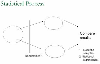
Students need to be strongly encouraged to read the Chapter Summary and the Technology Summary. Especially in this preliminary edition with no index, students will need to carefully organize their notes. You should remind them that this course will be rather “cyclic” in that these ideas will return and be built upon in later chapters. With these students, we have had good luck asking them to submit potential exam questions as part of the review process. You might also consider showing students a graphic of the overall statistical process and how the ideas they have learned so far fit in, e.g.:
This chapter parallels the previous chapter (considering of data
collection issues, numerical and graphical summaries, and statistical inference
from empirical p-values) but for quantitative variables instead of categorical
variables. The themes of considering the
study design and exploring the data are reiterated to remind students of their
importance. Analyses for quantitative
data are a bit more complicated, because no longer does one number summarize a
distribution and we focus on shape, center, and spread in describing these
distributions. This also leads to
heavier use of Minitab for analyzing data (e.g., constructing graphs and
calculating numerical summaries) as well as for simulations. If your class does not meet regularly in a
computer lab, you might want to consider having students work through the initial
study questions of several investigations, saving up the Minitab analysis parts
for when you can visit a computer lab.
Or if you do not have much lab access, you could use computer projection
to demonstrate the Minitab analyses. Keep in mind that there are a few menu
differences if you are using Minitab 13 instead of Minitab 14 (see the powerpoint slides for
Day 8 of Stat 212). One thing you will
want to discuss with your students is the best way to save and import graphics
for your computer setting. Some things
we’ve used can be found here.
Section 2-1:
Summarizing Quantitative Data
Timing/Materials:
Students will be using Minitab in Investigations 2-3 (oldfaithful.mtw), 2-5 (temps.mtw), and 2-6 (fan03.mtw). Instructions for replicating the output shown in Investigation 2-2 (cloudseeding.mtw) are included as a Minitab Detour on p. 92. Excel is used in Investigation 2-7 (housing.xls). Investigations 2-1 and 2-2 together should take about 50-60 minutes. Investigations 2-3, 2-4, and 2-5 together should take another 60 minutes or so. Investigation 2-6 could take 40-50 minutes, and Investigation 2-7 could take 50-60 minutes. You might consider assigning Investigation 2-6 as a “lab” that students work on in pairs and complete the “write-up” outside of class. Investigation 2-7 explores the mathematical properties of least squares estimation in this univariate case and can be skipped or moved outside of class.
Investigation 2-1 is meant to provoke informal discussions of anticipating variable behavior. You may choose to wait until students have been introduced to histograms (in which case it could also serve to practice terminology such as skewness). You can also consider using your own survey questions and having students examine their own data. It’s even entertaining to look at their own results after doing this activity and seeing whether the behavior at your school as the same as for the data provided. One goal is to help students get used to having the variable along the horizontal axis with the vertical axis representing the frequencies of observational units. Furthermore, we want to build student intuition for how different variables might be expected to behave. You will probably want to have students add identifying numbers to the graphs for easier reference:
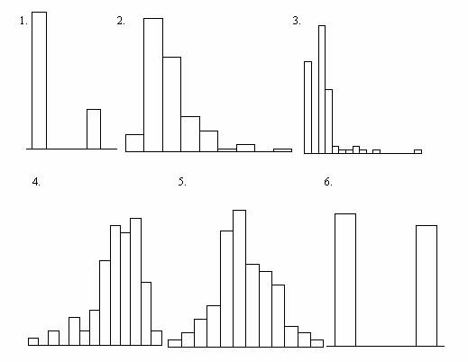
Students usually quickly identify graphs 1 and 6 as either the soda choice or the gender variable, the only categorical variables. Reasonable arguments can be made for either choice. In fact, we try to resist telling students there is one “right answer” (another habit of mind we want them to get into in this statistics class that some students may not be expecting, as well as that writing coherent explanations will be an expected skill in this class). We tell them we are more interested in their justification than their final choice, but that we see how well they support their answers and the consistency of their arguments. A clue could be given to remind students the name of the course these 35 students were taking. This often leads students to select graph 1 as the gender variable, assuming the second bar represents a smaller proportion of women in a class for engineers and scientists. Students usually pick graphs 2 and 3 (the two skewed to the right graphs) as number of siblings and haircut cost. We do hope they will realize that graph 3, with its gap in the second position and its longer right tail (encourage students to try to put numerical values along the horizontal scale) is not reasonable for number of siblings. However the higher peak at $0 (free haircuts by friends) and the gap between probably $5 and $10 does seem reasonable. (In fact, students often fail to think about the graph possibly starting at 0.) We also expect students to choose between height and guesses of age for graphs 4 and 5. Again, reasonable arguments could be made for either, more symmetric shape for height, as expected for a biological characteristic? Or skewed shape for height (especially if they felt the class had a smaller proportion of women)? Again, we evaluate their ability to justify the variable behavior, not just their final choice. This investigation also works well as a paired quiz but the habits of mind that this investigation advocates were part of the motivation for moving it to first in the section.
In Investigation 2-2 students are introduced to some of the common graphical and numerical summaries used with quantitative data, while still in the context of comparing the results of two experimental groups. We present these fairly quickly, and we emphasize the subtler ideas of comparing distributions, because we don't really want to pretend that these mathematically inclined students have never seen a histogram or a median before! This investigation concludes by having students transform the data. While not involving calculus, transforming data is an idea that mathematically inclined students find easier to handle than their more mathematically challenged peers. This piece can be skipped but there are later investigations that assume they have seen this idea. You might also consider asking students to work on these Minitab steps outside of class. Practice 2-1 may seem straight-forward, but some students struggle with it, and it does assess whether students understand how to interpret boxplots. It does not require use of Minitab, but Practice 2-2 does. In Practice 2-2, you might consider narrowing the focus to asking the students to pick just one comparison and asking if t he wood vs. steel comparison is in the direction expected.
Investigation 2-3 formally introduces measures of spread and
histograms. The data concern
observations of times between eruptions at
|
|
Jan |
Feb |
Mar |
Apr |
May |
Jun |
Jul |
Aug |
Sep |
Oct |
Nov |
Dec |
|
|
39 |
42 |
50 |
59 |
67 |
74 |
78 |
77 |
71 |
60 |
51 |
43 |
|
SF |
49 |
52 |
53 |
56 |
58 |
62 |
63 |
64 |
65 |
61 |
55 |
49 |
Practice 2-4 tries to convince students to consider a few different histogram bin widths to make sure they aren’t missing some detail. A related java applet can be found here. Investigation 2-5 aims to motivate the idea of standardized scores for “comparing apples and oranges.” While students may realize you are working with a linear transformation of the data, we hope they will see the larger message of trying to compare observations on different scales through standardization. Practice 2-7 should help drive this point home. You also want to reiterate to students that the “suprisingness” of a data value will depend on both the distance from the mean and the variability in the data. The empirical rule is used to motivate an interpretation of standard deviation (half-width of middle 68% of a symmetric distribution) that parallels their understanding of IQR. (See also the results of Practice 2-6.)
Investigation 2-6 gives students considerably more practice in using Minitab to analyze their data. Students will probably need some help with questions (n)-(p) especially if they are not baseball fans. These questions can be addressed in class discussion where those that are baseball fans can be the “experts” for the day. Still, we also want students to get into the mental habit of playing detective as they explore data. We find Practice 2-9 helps transition the data set to one that applies more directly to individual students. We encourage you to collect students’ written explanations (perhaps in pairs) to provide feedback on their report writing skills (incorporating graphics and interpreting results in context). If treated more as a lab assignment, you might consider a 20 point scale:
Defining MCI: 2 pts; Creating dotplots: 2 pts; Creating boxplots: 2 pts; Producing descriptive statistics: 2 pts; Discussion: 8 pts (shape, center, spread, outliers); Removing one team and commenting on influence: 3 points; Overall communication: 1 point (including embedding the graphics into the report). Such a rubric can be shown to the students as part of the assignment statement as well.
Investigation 2-7 leads students to explore mathematical properties of measures of center, and it also introduces the principle of least squares in a univariate setting. As we mentioned above, this investigation can easily be skipped. Questions (a) and (b) motivate the need for some criterion by which to compare point estimates, and questions (c)-(h) reveal that the mean serves as the balance point of a distribution. Beginning in (k), students use Excel to compare various other criteria, principally for comparing the sum of absolute deviations and the sum of squared deviations. Students who are not familiar with Excel may need some help, particularly with the “fill down” feature. Questions (o) and (p) are meant to show students that the location(s) of the minimum is not affected by the extremes but is affected by the middle. Students will be challenged to make a conjecture in (q), but some students will realize that the median does the job. Questions (t)-(w) redo the analysis for the sum of squared deviations, and in (x) students are asked to use calculus to prove that the mean minimizes SSD. This calculus derivation goes slowly for most students working on their own, so you will want to decide whether to save time by leading them through that. Practice 2-10 extends the analysis to an odd number of observations, and Practice 2-11 looks at a new criterion, the maximum of absolute deviations, for which the minimum occurs at the mid-range.
Section 2-2: Statistical Significance
Timing/Materials: Students are asked to conduct a simulation using index cards in Investigation 2-8, follow-up by creating and executing a Minitab macro. Encourage students to review the steps in creating a macro prior to coming to class. This macro is used again in Investigation 2-9 and then modified to carry out an analysis in Investigation 2-10. This section might take 75-90 minutes.
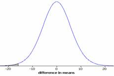
This section again returns to the question of statistical significance, as in Chapter 1, but now for a quantitative response variable. As before, students will use shuffled cards and then a Minitab macro to simulate a randomization distribution. However this time there will not be a parallel probability model, because we need to consider not only the number of samples but also the value of the mean for each sample which is computationally intensive. We encourage you to especially play up the context in Investigation 2-8 where students can learn a powerful message about the effects of sleep deprivation. (It has been shown that sleep deprivation impairs visual skills and thinking the next day, this study examines the effects 3 days later.) The tactile simulation will probably feel repetitive so you may try to streamline it but we have found students still need some convincing on the process behind a randomization test. It is also interesting to have students examine medians as well as means. In question (h) we again have students add their results to a dotplot on the board. Students are asked to type in the macro commands, you may also choose to provide the macro file to them. Either way, it will be important for them to understand what Minitab is doing. Remembering to initialize the counter (let k1=1 at the MTB> prompt) before running the macro is the most common error that occurs; students also need to be reminded that spelling and punctuation are crucial to the functionality of the macro. In this case, they also need to realize that the worksheet containing the data needs to be open before they run the macro. Indicator variables, as in (l), will also be used extensively throughout the book. We encourage students to get into the habit of running the macro once to make sure it is executing properly before they try to execute it 1000 times. We do show them the results of generating all possible randomizations in (p) to convince them of the intractability of this approach and to motivate later study of the t distribution. You might consider providing more feedback (e.g., collecting samples of their answers) for questions (d) and (e) to monitor students’ progress with these concepts. A slightly improved version of the figure on p. 128 is below:
Investigations 2-9 and 2-10 provide further practice while focusing on two statistical issues: the effect of within group variability on p-values (having already studied sample size effects in Chapter 1) and how to interpret p-values with observational data. Question (b) of Investigation 2-9 is a good example of how important we think it is to force students to make predictions, regardless of whether or not their intuition guides them well at this point; students struggle with this one, but we hope that they better remember and understand the point (that more variability within groups leads to less convincing evidence that the groups differ) through having made a conjecture in the first place. The subsequent practice problems are a bit more involved than most, so you may want to incorporate them more into class and/or homework.
In this chapter, we transition from comparing two groups to focusing on how to sample the observational units from a population. While issues of generalizing from the sample to the population were touched on earlier, in this chapter students formally learn about random sampling. We focus (but not exclusively) on categorical variables and introduce the binomial distribution in this chapter, along with more ideas and notation of significance testing. There is a new spate of terminology that you will want to ensure students have sufficient practice applying. In particular, we try hard to help students clearly distinguish between the processes of random sampling and randomization, as well as the goals and implications of each.
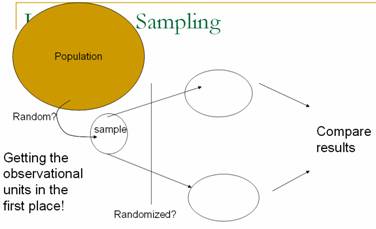
Section 3-1: Sampling from Populations I
Timing/Materials: Investigation 3-1 should take about one hour. A version of Table I (a random number table) has been placed here. Students can also use a random number generator in their calculator if you aren’t concerned that they learn to use a random number table (though the latter is convenient for testing situations). Investigation 3-2 can be done quickly at the end of a class period, about 15 minutes. An applet is used in Investigation 3-3 and there are some Minitab questions in Investigation 3-4. These two investigations together probably take 60-75 minutes. You will probably want students to be able to use Minitab in Investigation 3-5 which can take 30-40 minutes. Investigation 3-6 is a Minitab exercise focusing on properties of different sampling methods (e.g., stratified sampling) which could be moved outside of class (about 30 minutes) or skipped. Investigations 3-2 and 3-6 can be regarded as optional if you are short on time.
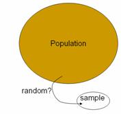
The goal of Investigation 3-1 is to convince students on the
need for (statistical) random sampling rather than convenience sampling or
human judgment. Some students quibble
that part (a) only asks for “representative words” which they interpret as
indicating representing language from the time or words conveying the meaning
of the speech. This allows you to
discuss that we mean representative as having the same characteristics of the
population, regardless of which characteristics you will decide to focus
on. Here we focus on length of words
expecting most students to oversample the longer
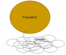
words. Through constructing the dotplot of their initial samples (again, we usually have
students come to the front of the class to add their own observation) we also
hope to provide students with a visual image of bias, with almost of the
student averages falling above the population average. We hope having students construct graphs of
their sample data prior to the sampling distribution will help them distinguish
between these distributions, and you will want to point this out
frequently. The sampling distribution of
the sample proportions, due to the small sample size and granularity may not
produce as a dramatic an illustration of bias, but will still help get students
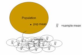
thinking about sampling distributions and sampling variability. This investigation also helps students
practice with the new terminology and notation related to parameters and
statistics. We often encourage students
to remember that the population parameters are denoted by Greek letters, as in
real applications they are unknown to the researchers (“It’s Greek to
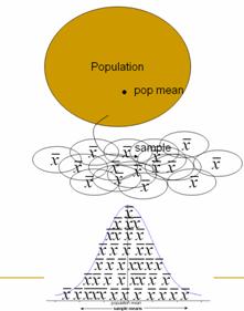
me!”). The goals of questions (t)-(w)
are to show students that random sampling does not eliminate sampling
variability but does move the center of the sampling distribution to the
parameter of interest. By question (w)
they should believe that a method using a small random sample is better than
using larger nonrandom samples. Practice
3-1 uses a well-known historical context to drive this point home (You can also
discuss
Investigation 3-2 is meant as a quick introduction to alternative sampling methods. You may even choose to talk students through these ideas but it’s important for them to consider methods that are still statistically random but that may be more convenient to use in practice.
Investigation 3-3 continues the exploration of samples of words
from the