INVESTIGATING STATISTICAL CONCEPTS, APPLICATIONS, AND METHODS, Third Edition

NOTES FOR INSTRUCTORS

August, 2022

Chapter 1 Chapter 2 Chapter 3 Chapter 4 Chapter 5

CHAPTER 4: COMPARISONS WITH QUANTITATIVE VARIABLES

This chapter focuses on comparing two groups on a quantitative variable. In Chapter 2, we already discussed explorations of distributions with quantitative variables and the sampling distribution of a sample mean, introducing the t-distribution and one-sample t-tests. We begin this chapter with a short (optional) investigation reviewing these ideas and statistical significance (where you can list out all possible assignments of observations to two groups). Following the structure of the previous chapter, we first discuss comparing two population parameters (modelling random sampling, Section 2) but then contrast that with comparing two treatment parameters (modelling random assignment, Section 3). In each case, we transition to t-procedures and you have some options of how much detail you want to include here. You will need to make some choices as to how many of these simulations you want students to carry out themselves vs. you demonstrating vs. you talking them through the concept. Section 4 looks at matched pair designs, through simulation and then through the paired t test. (By this point in the course, students can be asked to consider advantages and disadvantages of different analysis approaches. You can also tie back to discussion of the sign test in Chapter 2.) Investigation 4.10 also looks at paired categorical data through McNemar’s test.

Section 1: Comparing Groups – Quantitative Response

Investigation 4.1: Employment Discrimination?

We have moved this investigation into the main text from being an example. It is a context students should find engaging and we like the ability to think about “all possible assignments” of the observed response outcomes to the two groups. The main concepts to focus on are “conditioning on the outcomes” and that the “random assignment” here is purely hypothetical (and therefore the applicability of the p-value is even a little debatable). We prefer to allow students to consider this a “hypothetical” p-value – how unusual would the result had been had there been random assignment, as a measure of strength of evidence, being very cautious not to draw any causal conclusions. It’s also a good reminder that although the set-up is similar to a hypergeometric setting, we have to determine the actual value of the statistic each time, we can now longer simply count successes and failures as with categorical data.

We reworked this investigation a bit but you may want even more focus on listing out all the possible random assignments and the corresponding statistics and which you want to consider “more unusual.”

Section 2: Comparing Two Population Means

The following investigations have been reordered to better distinguish between taking independent random samples and using random assignment.

Investigation 4.2: The Elephants in the Room

Materials: The elephants data and the NBASalary2021.txt file. You may want to demo how to copy the data into Excel for extracting the columns of interest. You may also want to use the NBASalaries2021_2.txt file (which has already been cleaned and reports salaries in millions of dollars). Focusing on the Comparing Two Populations applet. (The corresponding R/Minitab/JMP macros have been moved to the end or you could have students write their own). Remind students that if they “select all” and copy and paste from the web page, they will have some extra “missing values” at the bottom of the file that they will need to remove.

The main goal of this investigation is to explore the sampling distribution of the difference in two sample means to justify use of the t-test. We start with a scientific study of elephant travel distances to motive the sample data. Then we have a “detour” where we have access to population data (the NBA salaries) to sample from. Once the simulation convinces students when a t-test is appropriate, they return to apply it to the elephant data. Hopefully the detour is not too much of a distraction and helps them differentiate (real data = no population information) vs. (have population = theoretical results). The first practice problem gives them an opportunity to compare their analysis with bootstrapping, the second focuses on the important impact of sample size.

The investigation also gives the opportunity to raise some interesting data exploration questions (e.g., mean vs. median, limitations of boxplots, reminders on interpretations of shape, center, and variability). Note: The ISCAM workspace boxplot does now use variable box widths for differing sample sizes.

For the detour, students can load in the population data (just salaries and conferences, which is easiest to do from NBASalary2021_2.txt). Students can then take independent random samples from these populations. If you check the Pooled box, the observations in each sample can come from either population. This would model the null hypothesis being true which is not needed for the detour. The applet also does not display a “statistic” for the population data. The applet does report population standard deviations. In (k), we want them to think about the non-normal data and the finite vs. infinite populations. Students then explore whether the t-distribution is well-approximated by the t-distribution without going into lots of details about pooled vs. unpooled SD and degrees of freedom. You may be able to move through this material fairly quickly as students should not be surprised at the development of the t distribution as an approximation for the sampling distribution. You also have options in how much time to spend on the derivation of the standard error; students should at least hear some intuition for why the variances add when looking at a difference. We focus on comparing the simulation results to the value predicted by the formula.

Students can then practice carrying out two-sample t-procedures with the elephant data. The result is not at all significant and this is a good time to remind them that absence of evidence is not evidence of absence. It might be worthwhile to have them interpret a confidence interval for the difference between two population means. We try to insist that they use language like “parameter 1 is XX to XX larger than parameter 2.”

Investigation 4.3: Left-handedness and Life Expectancy

Timing: Can be done in about 15-min or you can use the last questions as a jumping off point for further discussion about types of error.

Students will probably find this context interesting and it is worth spending some time talking about the data collection issues and the implications. The focus here is on the role of the nuisance parameters (population standard deviations) (this is also a good example of the common habit of many studies to report means but not sample standard deviations) and even the impact on the relative sample sizes of the two groups. We encourage you to ask students to make genuine predictions before performing any calculations. Make sure students take advantage of the technology (have them work in small groups) to complete these calculations fairly quickly so they can focus on the change in p-value. Students should do fairly well with (h) but we’ll see if they remember how to interpret standard deviation in terms of the 2SD rule (though should also keep in mind that lifespans are probably not symmetrically distribution).

You might also want to add confidence intervals to this investigation while they can truly interpret the parameter as a difference in population means.

Section 3: Comparing Two Treatment Means

In this section we focus on the random assignment as the source of randomness instead of random sampling. You again need to think about how much time to have students spend on the simulations, but we feel it can help distinguish the role of randomness. The tactile simulation here may help clarify the process more than in the previous section.

Investigation 4.4: Lingering Effects of Sleep Deprivation

Timing: 45 minutes

Materials needed: 21 index cards, Randomization Test applet

This is a similar situation to Investigation 4.1 but now random assignment was truly used in the study design and it is not feasible to list out all possible random assignments and calculate the statistic for each one, so we simulate a large number of random assignments instead. At this point, students may be able to walk you through how to design a simulation to explore the issue. You can focus on describing a tactile simulation or writing out “pseudo-code.” We think it is still worth the time to do a tactile simulation at this point. (Make sure everyone subtracts in the same way, deprived – unrestricted.) The applet has some nice visuals. It also allows you to easily change to the difference in medians but we now put off that discussion to the end of the chapter though you could preview it to show the flexibility of the randomization approach. You may also want to follow up the applet simulation with technology instructions for doing the simulated randomization distribution in R/Minitab/JMMP. The text also discusses the “exact” probability distribution and you can emphasize how cumbersome and really unnecessary it is to obtain that distribution. The simulation gives pretty close results and works for any statistic they choose to use.

In (b) you may want to emphasize a “schematic” of the experimental design.

Technology notes: If you plan to have them use R or Minitab or JMP for these simulations later (may not be necessary on top of the Randomization Test applet), be sure to have them save these scripts/txt files. Once students have seen the visual of the individual boxplots, you can remove that feature to speed up the simulation. You could also use the simulation results to try different df to see which t distribution provides the best/adequate fit to the simulated statistics.

Investigation 4.5: Lingering Effects of Sleep Deprivation (cont.)

This investigation continues the previous to motivate use of the t distribution with randomized experiments as well. The theoretical model gets a little sketchier here (e.g., not two independent random samples) and the goal is to convince students that the t model still works anyway. In the previous section we briefly discussed the concept of pooled vs. unpooled standard deviations. Pooling would make a bit more sense in the context of a randomized experiment, but again we ignore that option in favor of the more simplistic “never pool” approach. We try to convince students of the merit of the t distribution by showing the p-value is closer to the exact p-value. (Students probably won’t come up with this way of deciding on their own.) In (h), we ask them (!) how they want to define the parameter in this situation. We often use phrasing like “long run treatment mean” or “underlying treatment mean” and “for people like those in this study.” We think there is some value in discussing what the parameter represents, especially in the absence of random sampling, like for interpreting the confidence interval. This will play a larger focus in the next investigation.

It may bother students that the standard deviations aren’t more similar. If we truly had independent random samples from a larger population then

which we can estimate with =5.93. But in a randomization test, we are really treating the 21 observations as the population (so actually know ) and when we take 11 out to be group 1, we should apply a finite population correction. So . To find σ, we divide the sum of the squared deviations by 21 instead of 20. So with the sleep deprivation data, σ = 15.056, and = 3.21 and = 3.53 and so

with gives

» 6.74.

Investigation 4.6: Ice Cream Serving Sizes

Timing: 30 minutes

This investigation begins as review but carries through to the two-sample t-interval. Definitely let students know if there is a particular format you want them to use in interpreting these intervals (which may change depending on whether zero is included in the interval). You can also discuss the slightly nebulous nature of the parameter in such a randomized experiment, trying to reinforce the idea of their being some “true” or “long-run” mean response that you are estimating.

Investigation 4.7: Cloud Seeding

Timing: 60 minutes (You may want to collect the data for Investigation 4.8 during the preceding class period.)

Materials needed: Access to CloudSeeding.txt data file (stacked) and possibly the Comparing Groups (Quantitative) applet.

This investigation explores a random experiment with a very skewed response variable which brings into question the appropriateness of the two-sample t-procedures (though in Investigation 4.2 they already saw that the t-test is pretty robust, especially with similar shapes and sample sizes). Question (g) will probably be tough for them, but one approach is to consider using a statistic other than means, such as the more resistant median as a measure of center. You can draw the parallel with examining other statistics (like relative risk and odds ratio) at the end of Chapter 3. Students may also recall how we used a transformation to make a skewed distribution into a normal distribution in Chapter 2. You can then use technology to make this modification before analyzing the data. Students can easily calculate a p-value with the randomization test (remember to use the observed difference in group medians as the statistic), but what about a confidence interval?

Another approach is data transformation. As they saw before with a right skewed distribution the log transformation (rescaling) often works to “pull in” the larger values and create a more symmetric distribution. The last page also discusses back transforming the confidence interval into a ratio of population medians but you may not want to emphasize this detail with your students (though you can build on the multiplicative increase interpretation they used with relative risk and odds ratio). It is worth noting that the log transformation (essentially) preserves the median but not the mean.

Section 4: Matched Pairs Designs

The last section in this chapter focuses on paired data, both paired designs and analysis. Again students have an option for exploring a randomization approach to estimate the p-value. A good theme to emphasize throughout this section is the role of variability on our analyses, and how the statistician’s goals are to explain or at least account for as much of this variability as possible.

Originally Investigations 4.8 and 4.9 examined class-collected data on melting times of chocolate chips. This is a fun experiment that is easy to carry out during class. One caution is that the results do not always show the expected consistency in the repeated measures and in times of more social distancing, we replaced the context with one of swimming in guar (a syrupy substance) vs. water. The Mythbusters carried out the student which provides a fun video snippet, but did not provide much data. A 2004 article in American Institute of Chemical Engineers examined 16 swimmers though some of the data collection is unclear and some of the data values had to be inferred. In Fall 2021, a student project compared typing speeds with and without up-tempo background music. The data collection method appeared sound and the data performs nicely, with a much more significant result for the paired design. You could also ask students to take the typing test themselves, even if you don’t use the data for analysis. Versions of Investigation 4.8 and 4.9 using these data can be found here.

Investigation 4.8: Speed It Up

Timing: About 30 minutes, can start Investigation 4.9

Materials needed: None, but this replaced an activity asking students to melt semisweet and peanut butter chips, which is still a great data collection activity if feasible. Using an on screen timing mechanism for them to write down how long it took the chip to melt when held to the roof of their mouth. The chip data often does not show benefits of pairing however.

This investigation is based on a student project. You can have students try the same typing test. You can emphasize that “difference in means” is “mean difference,” but you really prefer the latter wording in this case and that the variability in these two quantities can be very different. This investigation motivates the need to reduce unexplained variation to increase the power of the comparison of interest. Much of this first activity will be intuitive for students. Make sure to give them some practice in identifying paired vs. independent samples, including matched pairs of individuals as well as repeated observations.

Investigation 4.9: Speed it Up (cont.)

Timing: About 30 minutes. If partway through, can probably combine with Investigation 4.10 in a 50-60 minute class period.

Materials needed: Matched Pairs Randomization applet

Now it’s time to estimate a p-value for the differences, based on a paired design. You will again want to have some caution in defining the parameter. In (g), you might want to see whether students can tell you how to design a simulation to mimic the randomness that was used in this study (the order of the tests), such as with a coin flip, assuming the typing speeds would have been the same no matter which condition they had. They may also be able to set up “pseudo-code” for the randomization. The Matched Pairs Randomization applet show them a visual of the speeds swapping places within each row before plotting the new differences and the average difference. (Another good time to highlight the distinction between population, sample, and sampling distribution.) It also allows you to see the “lines pattern” in the paired data to compare the observed “slopes” to the simulated slopes. The investigation then turns to the two-sample t-test and you can decide how much of the work you want the technology to do vs. having the students continue to focus on a one-sample t-test of the differences. You might also want to show the more general formula for the standard error of the difference in two sample means: 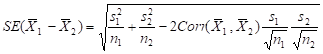and emphasize how the utility of pairing depends on how correlated the data are (though paired data should always be analyzed as such).

You need to decide whether your students need to be able to go back and forth between stacked and unstacked data.

Investigation 4.10: Comparison Shopping

Timing: 40 minutes, this can expand if you choose to do more with data cleaning and exploration

Materials needed: Optional - Access to shopping.txt (may also want to consider making this a class data collection project)

In R, you probably won’t be able to copy and paste from webpage (products with multiple names) but you can read.delim with the URL. You will also have to handle the missing values. This data set is small enough that they can be removed before importing into R. You can also remove them once in R (e.g., edit(x) or fix(x)), but for the paired data, you will need to remove them from all three columns. You will probably also need to convert them to numerical values using as.numeric. The following can convert the * values to NaN that R will recognize.

· For one set of values, the following will delete the missing values. The output is the same without na.omit but the sample size will not reflect the number of missing values.

na.omit(as.numeric(as.character(Luckys))))

· For paired data:

This induces NaNs in the columns.

combined=cbind(as.numeric(as.character(Luckys)),as.numeric(as.character(Scolaris)))

This deletes all of the rows that have a missing value for either store.

newcombined=na.omit(combined)

If you haven’t discussed different sampling plans yet, this is a good context. What would be problematic about taking a simple random sample of items and then finding their prices, if you have to wonder around an unfamiliar store? What would be an advantage to stratified sampling? Systematic sampling?

Once the data are cleaned (one of the few times we have a reason to remove an outlier – we can see that the items were not identical), the analysis is straight forward (though may also want to raise the issue about what to do when an item is on sale). So then the investigation turns to the idea of a prediction interval. Emphasize to students that they have created an interval for the population mean, not for individual items. (At this point, many students will still have this misconception or that the confidence interval captures 95% of sample means.) But they can create an interval for individual items if they take into account the additional item to item variability (in addition to the sample to sample variability). Be sure to clarify to students how you would phrase an exam question in each case.

A follow-up to this investigation could look at a sign test on the positive/negative differences, which would be resistant to outliers in the data but would lose power by ignoring the magnitude of the differences.

Investigation 4.11: Smoke Alarms

Timing: 30 minutes

Continuing the theme of pairing, this investigation does so again but with categorical data. Students should be able to see the intuition behind using a binomial test on the number of pairs where the outcomes differed, providing a nice review of earlier material.

Fall 2015: We streamlined this activity a bit by removing the simulation questions. Students should be able to see that reversing the observations often doesn’t change things and we focus on the observations that had a difference in response. We also focus the two-way table to be on the two variables recorded on each child.

Again, remind students of the end-of-chapter materials. Example 1 has them compare the different analysis options on the Westvaco employment discrimination data.

We have updated a few of the homework exercises, particularly the Wimbledon data set. For more discussion of some of these analytics see

http://bjsm.bmj.com/content/40/5/387

http://fivethirtyeight.com/features/why-some-tennis-matches-take-forever/