INVESTIGATING STATISTICAL CONCEPTS, APPLICATIONS, AND METHODS, Third Edition

NOTES FOR INSTRUCTORS

August, 2022

Chapter 1        Chapter 2 Chapter 3 Chapter 4 Chapter 5

Some features of the textbook you may want to highlight on the first day of class and discuss with students include:

· how to make the most use of include the glossary/index,

· links to applets and data files,

· study conclusion boxes, and

· errata page.

You should make sure students have access to the materials every day, either on their personal device (e.g., laptop or iPad) or printed out, as they will want to add notes as they go along. You may also want to insist on a calculator every day. You will also want to make sure they have detailed instructions for the technology tools you want them to use in class (e.g., R or Minitab or JMP), and ability to run javascript applets which should run on all platforms including mobile devices). In particular, you will want to make a direct link to the ISCAM.RData workspace file available to R users or to the JMP journal file for JMP users. They can follow these links to directly open the software and have access to some prewritten functions that make use of R/JMP much simplified. In particular, the JMP journal file includes direct access to the probability distribution calculator, common one-sample and two-sample inference procedures and common preference settings. (Students may need to download the JMP file to their computers first.) The R functions are often updated (e.g., now include variable width boxplots, slightly nicer graphics) so is worthwhile to use the link rather than download the file only. The R commands are purposely simple rather than requiring additional downloads if possible (and also not taking advantage of many new R features like the tidyverse). If you are using an R or Minitab or JMP-only version of the text, there will still be occasional mentions of the other package. You can use this as a reminder to students that there are other options, but generally ignore them.  If using the pdf files, you should be able to copy and paste commands from the pdf into the technology. One newer applet feature – if you know the name of the data file, you can often type the name of the file in the data window and it will load it in rather than copying and pasting from a webpage.

Investigations A and B

Although a major goal of this text is to get students to complete a statistical investigation as early in the course as possible, we find taking a few days at the beginning to overview some key ideas (namely distribution, variability, and probability) can be helpful.  We offer two investigations, which can be done inside or outside of class and in varying levels of details and in either order, to explore these ideas.  In particular, we now introduce/review the formula for a standard deviation in these preliminary investigations. We hope this will help the first discussion of standard deviation in the context of a null distribution easier for students to understand.  One more abstract idea you may want to emphasize from these first two investigations is the concept of a random process. You can even differentiate between a census (Investigation A) and an on-going, potentially infinite process (Investigation B).  You may also choose to have them do a more involved data analysis or other simulation models as follow-up before proceeding (e.g., see Chapter 0 Exercises).

Investigation A: Is My Water Safe?

Materials: You may want to share some of the news articles with students.

Timing: As a class discussion, this investigation takes 30-45 minutes. You should have time to review the syllabus and/or delve deeper into some of the ethical issues. Encourage students to explore the data on their own afterwards.

This is intended as a guided activity, but you may want to ask students to work together on individual questions at different points along the way. One of the main goals is to introduce students to some of the terms they will use every day in the course, to remind them that variables can be measured different ways as well as the importance of careful measurement of variables. There is minimal material on dotplots, and describing the distribution of a quantitative variable. You may want to spend more time here depending on your students’ background, but we encourage you to not spend too much time, these ideas will return quite often later in the course. In particular, many students may struggle with the idea of standard deviation. Caution them not to focus on the calculation, but as long as they can look at graphs and decide which has more variability in terms of “width” of the distribution, they have an appropriate understanding for this stage of the course. Depending on time, you could also do more with the idea of percentile.

You will want to highlight the study conclusions box for students and tell them how to use them throughout the course. Similarly, you can discuss how/whether you plan to use the practice problems at the end of each investigation.

Investigation B: Random Babies

Materials: Index cards (4 per student or pair of students).  Calculators. Random Babies applet.

An alternative “lab version” of the Monty Hall problem.

Timing: This can be used as an initial or “filler” exploration that focuses on the relative frequency interpretation of probability and using simulations to explore chance models.  One key distinction you might want to emphasize for students is the estimated probability from simulation and the exact probability found analytically, which is not always so straight forward.  There is also a tremendous amount of flexibility on how deeply you want to go into probability rules, expected value, and variance.  Many students don’t have a good understanding of what is meant by “simulation” so you may want to highlight that as you will return to the concept throughout the course. (You may even want to follow-up with additional simulation exercises, see Ch. 0 homework.) If you do the first part of this investigation in class, you probably want students bringing calculators as well.  For the hands-on simulation, bring four index cards for each person or pair of students.  You may want to watch/highlight use of the terms repetition vs. trial. A simpler case practice problem has been added. (Note: If you use the applet for other than four babies, you will not see the animation.)

For question (r), we encourage you to show students a visual representation as well, mapping each outcome in the sample space to a value of the random variable.  Then in discussion the E(X) formula, can show a weighted average and how the weights (relative frequencies) converge to the theoretical probabilities. There is also brief discussion around V(X) and we encourage you to emphasize why variability is an important consideration as well as the distinction between variability in data and variability in a random process.

Chapter 0 HW Exercises

Exercises 1-7 follow up Investigation A and Exercises 8-11 follow up Investigation B. There are some interesting contexts which you can return to later in the course. You might always want to give them some “messier” data sets to work with.

CHAPTER 1: ANALYZING ONE CATEGORICAL VARIABLE

Section 1: Analyzing a Process Probability

This section will cover all the big ideas of a full statistical investigation: considering the research question, describing data, stating hypotheses, tests of significance, confidence intervals, power, and scope of conclusions.  (Ideas of generalizability are raised but not focused on until later but you can bring in lots of statistical issues, like ethics, data snooping, types of error.)  Once you finish this section, you may want to emphasize to students that the remaining material will cycle through these approaches with different methods. (In fact, you may want to reassure students that you are starting with some of the tougher ideas first to give them time to practice and reinforce the ideas.)

Investigation 1.1: Friend or Foe?

Materials: You may want to bring some extra coins to class and/or tell students to in advance. The One Proportion Inference applet is javascript and should run on all platforms. The applet initially assumes the coin tossing context for  = 0.5 but then changes to spinners and “probability of success” more generally once you change the value of the input probability.  We encourage you to show some videos detailing the experiment, which can be required viewing prior to class.

Nature article Supplementary Information page

Overview video from Mind in the Making - The Essential Life Skills Every Child Needs, by Ellen Galinsky

UBC Center for Infant Cognition Lab website

Yale Social Evaluation page (needs QuickTime plug in)

Three specific videos: Triangle helps, Square hinders, 10-month old chooses

Fall 2020: Here is a “lab” version of this investigation.

Timing: The entire activity takes about 80 minutes. A good place to split up the activity is after the tactile simulation (part (k)). You can then assign them to review the Terminology Detour before the next class.  Technology instructions for tallying the outcomes and construct bar graphs are included, these can also be moved outside of class.

We find this investigation a very good entry to the big ideas of the course.  We encourage you to build up and discuss the design of the study (e.g., show the videos) and highlight the overall reasoning process (proof by contradiction, evidence vs. proof, ruling out "random chance" as a plausible explanation, possible vs. plausible).  Try not to let students get too bogged down in the study details (e.g., the researchers did rotate the colors, shapes, left/right side presentation, we are "modelling" each infant having the same probability, these infants may or may not be representative of all infants, etc.). 

In question (c), you can emphasize that examining a graph of the observed data is our usual first step. In question (e), it works well to get students to think for themselves about possible explanations for the high number picking the helper toy. They can usually come up with: there is something to the theory or it was a huge coincidence.  Now we have to decide between these explanations, but the random chance explanation is one that we can investigate. Maybe ask them how many infants would need to pick the helper toy for them to find it convincing. Depending on your class size, you may ask them to do more or fewer repetitions in question (i).  You can also ask them to predict what they will see in the dotplot before it’s displayed. Try to give students time to work through the applet and begin to draw their own conclusions. It will be important to emphasize to students why you are looking at the results for  = .5, and how that will help address the research question. Students can usually get the idea that small p-values provide evidence against the “random chance alone” or “fluke” or “coincidence” explanation, and then warn them you will refine that interpretation as the course progresses. (But may want to highlight for them what the random component is in their probability calculation.) As you wrap up the investigation you will want to focus on the reasoning behind the conclusion and precise phrasing of the conclusions.  In particular, you may want to emphasize the distinction between interpreting the p-value and evaluating the p-value.  The strategy outlined in the Summary gives a nice framework to the process (statistic, simulation, strength of evidence). You will especially want to repeatedly emphasize how the p-value is calculated assuming the null hypothesis is true. You may want to emphasize the “tail area” aspect of the p-value as a way to standardize the measurement of what’s unusual across different types of distributions (e.g., if we had a large sample size than any one outcome would have a low probability). You may want to poll a few students to report the p-value they estimated from the simulation to see that they vary slightly.  This may motivate some students to want to calculate an “exact” answer that everyone should agree on, and this is certainly possible using a bit of probability theory.

Make sure to ask students lots of questions on the reasoning process. We have emphasized that p-values are just one way of measuring how extreme an observation is in a distribution and tried to improve the motivation for “or more extreme” in its calculation.

Technology: The data files and applets page includes a link to “raw data” and you might want to get their feet wet reading the data in from a webpage or a URL (see Technology Detour). 

· With Minitab, you can copy and paste from the webpage into the data window (but watch that an extra missing value is not added to the end of the column).  You may want to introduce them to the “commands” window in case they want to copy and paste earlier instructions rather than using the menus/save the commands for documentation.

· With JMP, you can copy and paste from the webpage into the data window (but watch that you include the column headings). 

· With R, you can copy and paste the data onto the clipboard and use read.table. With data files, you use read.table (tab delimited) or read.csv (for comma delimited). With R Studio, you can use Import Data > From Text (rear). With R Markdown, you can use:

```{r}

Infants <- read.delim("http://www.rossmanchance.com/iscam3/data/InfantData.txt")

load(url("http://www.rossmanchance.com/iscam3/ISCAM.RData"))

```

to load in (tab delimited) data and the ISCAM workspace. You can tell students how to “attach” their data rather than referencing (e.g., data = ). This is ok for a first course that typically uses one dataset at a time.  To convert the * values to NaN, you can use as.numeric(as.character(x)).  Also make sure students see the question mark features with R and with the iscam R functions and/or the auto-fill feature in RStudio.

For the simulations, the text generally defaults to 1,000 trials, but you should feel free to mix that up a bit as well or occasionally do more just to make sure the answer is “stable.”

Investigation 1.2: Can Wolves Understand Human Cues

Materials: The journal article has some nice/helpful pictures of the experimental set-up. You can also easily access the data for the other animals.

Timing: This investigation is new for Fall 2022, but we predict it will take about 45 minutes.

The main focus is on calculating binomial probabilities, so you have some flexibility in how much detail you want to cover. We like this context (repeated measurements on one wolf) to be a good application of a binomial process, which introducing some basic terminology to follow up the reasoning from Investigation 1.1. This investigation doesn’t introduce any symbols yet but does try to help students make a detailed interpretation of the p-value. This is also a good place to practice the structure of a “simulation model” which can choose to return to several times in the course. We find emphasizing the distinction between “real data” and “hypothetical data” to be useful. This investigation also allows you to draw the distinction between the simulated p-value and the exact p-value.  Having 2-3 methods for finding the p-value (exact vs. simulation vs. normal-model) will be a theme throughout the book.  Another issue that you may want to emphasize but may take getting used to is always defining the parameter as a process probability (rather than a population proportion). You can also have good discussions on what p-values consistent sufficiently strong evidence.

Practice Problem 1.2B is a great follow-up using data you collect (in advance) on the students. link to the pictures can be found here. We have tried randomizing the order of the faces/choices and have not found that to affect the results (but you may want to incorporate this into your data collection as well).  A google docs type survey for collecting student responses can work well here. Please email me if you are interested in an online lab version of the matching names to faces study.

Technology: Students work through the technology instructions on their own. In Investigation 1.2, the technology instructions focus on calculating binomial probabilities. In the Investigation 1.4, they will see how to incorporate this into the more “complete” binomial test commands.

Investigation 1.3: Are You Clairvoyant?

Materials: You can use the One Proportion Inference applet and/or statistical software to calculate probabilities from the binomial distribution and/or a formal binomial test.

Timing: 45 minutes, especially if you have them self-test their clairvoyance before coming to class.

We felt students could use a bit more practice with binomial calculations, as well as a distinct introducing as the symbol for an unknown process probability, and introducing standardization as an alternative measure of extremeness. Students can play with an online version of the clairvoyance test (predicting what’s going to happen) before hand and/or you can do a quick demonstration or have them test each other’s ESP with actual cards in class. We do think it’s useful for students to analyze their “own” data once in a while, though here we suspect most will not find a significant difference, and the result may not even be in the conjectured direction (good time to talk about p-values > 0.50). The investigation presents E(X) and SD(X) but you could point them to this page that explains a bit more about where those expressions come from. By the end, we would like students to have in mind “less than 5% of the time” or “more than 2 standard deviations away” as unusual observations. (Although z-scores won’t be used in more detail until they look at the normal approximation to the binomial.) You may need to remind students that variance is standard deviation squared.

Be sure to highlight the distinction between the unknown parameter and a conjectured value for the parameter, as well as the distinctions between parameter, statistic, and variable. You will also want to emphasize whether you are going to ask students to distinguish an interpretation of the p-value (what does it measure) from an evaluation (of the p-value, deciding whether it is small).

Technology note: Students will be learning several different ways to do these calculations the first few days. You may want to move some of these calculations outside of class and have them submit their numerical answers between classes, but we mostly encourage you to let the technology handle the tedious calculations from this point on. 

· For the ISCAM workspace functions, initially they are told to use the lower.tail feature, mimicking the more generic R functions, but then they will switch to “above/below” type inputs. (Some instructors prefer going straight to iscambinomtest.)  Be sure to emphasize some of the subtle issues in R, like punctuation, continuing on to another line, short-cuts in the inputs, capitalization matters, etc.).  You could use binom.test in R but again we prefer the automatic picture.

· Many of the iscam R functions return key values for you to access individually, for example

> results=iscambinomtest(observed=14, n=16, hyp=.5, alt="greater")

will store the p-value and the endpoints of the confidence interval:

> results$pvalue

The confidence level inputs can also usually be either the decimal (.95) or the percentage (95) or a vector (c(.95, .99)). The return values are especially useful for R Markdown (e.g., embedding the result into text), e.g., This p-value of `r myresults$pvalue`…

Investigation 1.4: Heart Transplant Mortality

Timing: This investigation is mostly review and may only take 30-45 minutes.

This investigation provides additional practice (but with a hypothesized probability other than 0.5) and highlights the different analysis approaches.  Try to get students comfortable with the overall reasoning process but that there are alternative reasonable approaches to obtaining a p-value. You may want to focus on Ho as the "by chance" hypothesis (ho hum) and Ha as the research conjecture (a ha!). Also emphasize the distinction between St. George's (underlying) death rate and the observed proportion of deaths and the 0.15 value. You may want to emphasize the statistical thinking underlying this investigation – e.g., how we really shouldn’t reuse the initial data in testing the theory that the data pointed to (see also question q).  So ethnical issues, as well as the role of sample size, can be emphasized in discussing this activity. Students may struggle a bit with seeing these observations as a sample from some larger process with an underlying probability of “success.”  Students will appreciate defining “death” as a “success” as is common in many epidemiological studies.  The text also draws their attention to “failing to reject” null hypothesis versus “accepting the null hypothesis.”

The graphs of the two binomial distributions provide an opportunity to discuss how the mean, standard deviation, and shape of the binomial distribution change with the sample size. In (p), we are hoping students may notice the difference in the granularity of the distributions as a precursor to the normal approximation and the need for a continuity correction.  Students may also suggest the difference in the scaling of the vertical axis which is a related idea and also ties into the motivation for “or more extreme” in calculating a p-value that can be compared across distributions. You will also want to strongly emphasize that p-value calculations take sample size into account.  So a small p-value should not be discredited by a small sample size.

Technology notes: The One Proportion Inference applet does have the option for showing the summary statistics (mean and standard deviation) of the simulated values, but we advise not to pay much attention to those details yet.  You can also input only the probability of success, sample size, and value of interest, (press the Count button), and continue directly to the check the Exact Binomial box. You may want to use R or another technology that reports the binomial probabilities to more decimal places so they can see the exact equivalence in question (g). Students may wonder about the distinction between “calculating a binomial probability” and “carrying out a binomial test”; you may want to give them a diagram of the steps you want included whenever you ask them to carry out a test (of which finding the probability for the p-value is a middle step).

This includes introducing them to formal “binomial tests” (but emphasize this is just doing in one step what they had done previously).

· In R, the materials make use of iscambinomtest which gives the output and graph together. You may also want to compare this output to R's standard binom.test. You could of course use pbinom (e.g., 1-pbinom(13, 16, .5, TRUE) or pbinom(14, 16, .5, FALSE)), but we prefer the iscam function which includes the graph and uses non-strict inequalities for both tails.

· In JMP, we recommend asking students to download the Distribution Calculator for use throughout the course. They can download it to their Desktop and simply double click on it in the future. You will also want to consider this option in a lab environment. You will need to be careful in finding non-strict greater than probabilities with discrete random variables. In JMP, if you only enter one probability that outcome is defined as “success.” Otherwise JMP assumes “success” to be the first category alphabetically unless you specify otherwise with Column Properties > Value Ordering.

· In Minitab, the Probability Distribution Plot feature is advantageous in ease of use and including a visual of the (shaded) probability distribution. You may want to ask students to double click on the axis label to change the text to something more descriptive.

Investigation 1.5: Butter-Side Down Again?

Materials: There are some videos of the episode online, including some free “trailers” but you may have to pass some ads. The “butter-side down again?” is a quote from one of the videos. You can also emphasize the processes that the Mythbusters went through before collecting their final data.

Timing: 30 minutes depending on how much time you want to spend on two-sided p-value calculations

The main goal is introducing a “not equal to” research question where the researchers have no prior suspicion or specific concern as to the direction of the alternative hypothesis. You will want to emphasize that this distinction needs to be made before the data are collected (and in fact, the Mythbusters did have the direction wrong, though do watch for the distinction between falling off a table and falling from the roof of a building). Students will have good initial intuition for “checking the other side,” but the idea of “smallest p-value” will be more difficult and you may want to emphasize recognizing a two-sided alternative hypothesis and then conveying that information to the software. It is probably not worth spending much time on the "method of small p-values" other than to warn students that different packages may use slightly different algorithms.

Practice Problem 1.5 follows-up with their pilot test to develop the “unbiased” dropping mechanism in the first place. Here the Mythbusters did draw an erroneous statistical conclusion, thinking that 3 out of 10 was outside a statistical sample. You could encourage students to write their explanations in language that the hosts could understand.

Investigation 1.6: Kissing the Right Way

Materials: Tic Tac candy advertisement

Timing: 45 minutes, depending on how much time you give students to develop the interval themselves or crowd-source the information (e.g., assigning each pair of students on value to check out)

The transition here is to estimate the parameter vs. only testing one specific value. You may want to build up this “second inferential approach” more than the text does and how confidence intervals are really as, if not more informative than the tests. Do encourage students not to think of a CI as “new evidence” but more a different way of looking at the same evidence. This investigation introduces students to the concept of interval estimation by asking them to construct a set of plausible values for the parameter based on inverting the (two-sided) test. In (f),are hoping they will mention as an obvious first choice. Students often like to get into the “game” of seeing how close they can find the p-value to the cut-offs. The goal is also for students to see how that p-value changes as the hypothesized parameter moves away from the observed proportion (the R output provides a nice illustration of this but will need to be discussed with the students) and also the effect of the confidence level on the interval.  You may want to emphasize that the “inversion” necessary for these binomial intervals is actually pretty complicated and ends up being conservative because of the discreteness (when you plug in 0.05, it will return a value where the probability is at least 0.05). 

You may want to emphasize the distinction between “do a majority lean left” (which would be one-sided) and “how often do couples lean left.” You can also highlight properties of confidence intervals (e.g., widen with confidence level, shorten with larger sample size), but these ideas will definitely come up in the Section 2 as well.

Technology: The One Proportion Inference applet includes a slider for the process probability (and one for the sample size). You may still want students to do the first chart in (c) “manually” and then move to the slider in (d).

The R functions (binomtest, onepropz, twopropz, onesamplet) allow you to enter multiple confidence levels, e.g., iscambinomtest(11, 20, conf.level = c(.90, .95)) to display the intervals together in the output window. 

Option: You could begin Ch. 2 through the normal distribution before Section 2.

Section 2: Normal Approximation for Sample Proportions

This section reviews the previous material but through the “traditional” computational model – the normal distribution. The audience for this course is typically capable of working with the normal model without a lot of background detail, but some background will be helpful when you get to critical values and if you cover the continuity correction ideas. (You may want to detour with some traditional normal probability model calculations for practice.) Try to emphasize the parallels with the previous methods (simulation, exact binomial), the correspondence between the binomial and normal results, and some tongue-in-cheek that these normal-based methods aren’t really necessary anymore with modern computing. Although students may appreciate the simplification in some of the calculations, in particular how to improve the calculation of confidence intervals.

Investigation 1.7: Reese’s Pieces

Timing: This activity is now optional and really only here if your students need additional practice thinking in terms of distributions of proportions.

Technology Note: There is also an option for more M&M like colors (see link at bottom of page).

The beginning of this activity is largely review, but students will appreciate the candies.  The fun size bags of Reese's work well, or you can bring dixie cups and fill them up individually.  (Do watch for peanut allergies.) We would continue to stress the distinction between the sample data for each student (e.g., the bar graphs) and the accumulated class data (the sampling distribution). You may want to adopt a catchy term for the latter distribution such as "what if" (what if the null had been true) or "null" distribution.  (We use "could have been" to refer to an individual simulated sample in these early investigations but not throughout the course.)

The applet transitions to focusing on using the sample proportion as the statistic and some advantages (and lack of changes) in doing so. In particular, the role of sample size and the commonality of the shape of the null distribution. You can also refer back to the end of Investigation 1.1 to motivate the formula for the theoretical standard deviation. With candies in hand, they may have the energy for (h). We definitely recommend showing the correspondence between the simulation results and the theoretical results for the mean and SD. You may want to briefly discuss the “2SD rule” and a great time to connect that with the 5% cut-off they may be used to using. You may also want to emphasize that this is an “interval” for sample proportions if you know (to help contrast later with a confidence interval for ).

The Reese's applet has a feature that displays the normal distribution’s probability value as well.  That visual will help emphasize the continued focus on how to interpret a p-value in terms of the percentage of samples with a result at least that extreme (under the hypothesized probability). You may also want to assign homework that has them look at how the SD formula changes (e.g., play with derivatives) with changes in n and  (especially maximizing at  = 0.5).

You may also want to detour to general practice with normal probability calculations for quantitative variables (example Canvas module), or wait until Chapter 2.

Investigation 1.8: Halloween Treats

Timing: 45-60 minutes, especially if they are familiar with the study context in advance (you might even want to assign parts (a)-(c) to be completed before class). You also need to decide how strongly you want to cover the continuity correction.

This investigation provides practice in using the Normal Distribution for calculating probabilities of sample proportions, including in the context of a two-sided p-value and the (optional) continuity correction. Continue to focus on interpreting the calculations. You may need to spend a few minutes justifying the use of the normal model as an alternative (approximate) model and the z-score provides one advantage and confidence intervals will provide a strong second one (and later power calculations).  Math majors will also appreciate seeing how the factors affecting the p-value show up in the z-score formula. Make sure they see the link to Ho and Ha (and ₀). You can also discuss why the z value is positive/negative and the short cuts they can take with a symmetric distribution. The term “test statistic” is new here, but you can link back to earlier discussion of standardizing.

You will have to caution them against "proving" the null and also that they are talking about the process in general vs. individual children.  You may want to try to get them in the habit of telling you the inputs to the technology they are using.

It is pretty amazing how much the continuity correction helps and you will want to refer to pictures in explaining it. Make sure students understand when you add or subtract the correction term, but otherwise you may not want to spend much time on the correction. (The Theory-Based Inference applet has a check box for this correct, adjusting both the z-value and the p-value.) It does force them to think deeply about many of the earlier ideas in the course (e.g., continuous vs. discrete and shape, center, and spread, strict inequalities). 

The practice problems focus on applying the normal approximation to other context and be sure to emphasis some cases (e.g., St. George’s hospital) where this may not be appropriate. Make sure students don’t miss the study conclusions box and the overall Summary of One Proportion z-test box.

Investigation 1.9: Kissing the Right Way (cont.)

Timing: 45-60 minutes

This investigation introduces the one proportion z-interval and you have some options as to how much detail you want to include (e.g., finding percentiles). Students may need more guidance in coming up with critical values. You will also want to discuss how this interval procedure relates to what they did before and to the general ± 2 SD form. (This will hopefully provide some motivation for the normal model.) They will need some guidance on question (d) and how we can think of 2 standard deviations as a maximum plausible distance. Students seem to do well with this “two standard deviation rule.” Try to get students to think in terms of the formula in (h) versus a specific calculated interval.

Not clear how much time you want to spend on sample size determination but student intuition here can be rather poor. Also, if not covered before, they will need to realize that the SD formula is maximized when the proportion equals 0.5. In the end, you may want to be a bit open in what they choose to use for  (e.g., 0.645 from the previous study or 0.5 to be safe, or both and contrast, or their own guess). 

If you have extra time, you may want to introduce the Simulating Confidence Intervals applet here to help them interpret “statistical confidence.” It works best to generate 200 intervals at a time and then accumulate to 1000.  Also have them think about what it means for the interval to be narrower - what that implies in response to the research question.  It can be nice to show how the binomial intervals are a bit longer and not symmetric. You will also need to decide how much emphasis you want to put on the frequentist interpretation of confidence level and the idea of “reliability” of a method.  Students will need lots of practice and feedback, even in recognizing when the question asks about interpretation of the interval vs. interpretation of the confidence level.

You may also want to make them think carefully about the difference between standard deviation and standard error at this point (Practice Problem 1.9B(b).

Investigation 1.10: Hospital Mortality Rates (cont.)

Timing: This can be done in combination with other activities and may take 15-30 minutes (it can tie in nicely with a review of the Wald interval and Wald vs. binomial intervals and how to decide between procedures).  You may have time at the end of a class period to collect their sample data for the first part of the next investigation (choosing 10 “representative” words).

Materials: You could also use student collected data here (e.g., left-handers, vegetarians) though be careful as to how you define the random process in that case.

Many statisticians (and JMP) now feel only the “plus four” method should be taught. We prefer to start with the traditional method for its intuition (estimate + margin of error) but do feel it’s important for students to see and understand the goals of this modern approach.  You can also highlight to students how they are using a method that has gained in popularity in the last 20 years vs. some of their other courses which only use methods that are centuries old. Make sure students don't get bogged down by the numerous methods but gain some insight into how we might decide one method is doing “better” than another or not. 

Do make sure you use 95% confidence in the Simulating Confidence Intervals applet with the Adjusted Wald – it may not use the fancier adjustment with other confidence interval levels. (It’s also illuminating to Sort the intervals and see the intervals with zero length with  = 0 for the Wald method.) Then let them practice on calculating the Adjusted Wald in (g), making sure students remember to increase n in the denominator as well as using the adjusted estimate. You may also want to assign a simple calculation practice for a practice problem to this investigation or focus on benefits/disadvantages of the procedures.

Investigation 1.10: Ganzfeld Experiments

We have replace the old “batting averages” context with this one that make easier use of the normal approximation, though we suspect there is still a better connection to student intuition with the batting averages context. This investigation uses the Power Simulation applet and then at the end provides the ability to confirm the calculations with different technology tools (which may or may not allow you to toggle between binomial and normal probabilities). We did find the “baggage” of “observed level of significance” problematic with the binomial case, but do provide one question at the end where they should switch back to binomial and you may want to discuss the unfortunate consequences of the discreteness of that distribution. The emphasize here should be on the definitions and reminding students that they already know how to make these calculations, it just becomes a two-step process.

Lots of practice problems here depending on whether you want to emphasize the definitions, the relationships, the visuals, or the calculations.

Section 3: Sampling from a Finite Population

There is a transition here to focusing on samples from a population rather than samples from a process. It may be worth defining a “process” (like coin tossing, or measurements from a stream) for them to help them see the distinction. The goal is to help them quickly see that they will be able to apply the same analysis tools but now we will really consider whether or not we can generalize our conclusions to a larger population based on how the sample was selected.

Investigation 1.12: Sampling Words

Timing: About 30 minutes and can probably be combined with 1.13 in one class period.

Students may not like the vagueness of the directions and you can tell them that you want the words in the sample to give you information about the population. In fact, we claim that even if you tell them you are trying to estimate the proportion of short words, you will still get bias.  We recommend getting students up and out of their seats to share their results for at least one of the distributions. In R, if using the ISCAM workspace in a lab, do be cautious that everyone may have the same seed! (You can remove the seed first.). Earlier we said we were most interested in the standard deviation of the simulated distribution. Here you can contrast with focusing on the mean for judging bias.

A nice extension to this activity if you have time is to consider stratified sampling and have them see the sampling distribution with less sampling variability (see Chapter 1 Appendix for brief introduction to this idea). Note: If multiple columns are pasted into the Sampling Words (Sampling Quantitative Variable) applet, categorical variables can be selected as stratifying or clustering variables. The computer will stratify based on population proportion. User needs to specify desired number of cluster. Bad choices can lead to poor results.

For practice problem 1.12A, consider whether or not you want students to write out the explanations for their answers.  You might also again emphasize the distinction between the distribution of the sample and the distribution of the sample statistics.

Investigation 1.13: Sampling Words (cont.)

We have tried to streamline the discussion of finite population correction factor, wanting to raise students awareness of the issue but then also how we usually get to ignore it.

This works well as a class discussion. You will want to again emphasize to students that this is one of the rare cases where we have the entire population and our goal is to investigate properties of the procedures so that we can better understand what they are telling us in actual research studies.  You will also want to empathize with students how counter intuitive the population size result is.  You can also remind them of the parallels to sampling from a process.

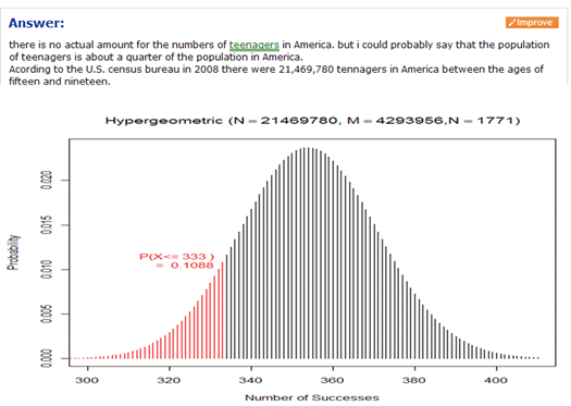
Investigation 1.14: Teen Hearing Loss

Timing: 15 minutes

This investigation again provides practice with the new terms and gets students back to the inferential world. You may want to compare the binomial calculations with the “exact” hypergeometric calculations, and even show the insensitivity of this calculation to the population size if the population proportion is held constant.

Investigation 1.15: Counting Concussions

This is student project data where a finite population correction is necessary. You could just highlight that feature as well as the definition of non-sampling errors if you haven’t yet. You will also want to think about whether you want to cover the hypergeometric distribution here or wait for the more intuitive use with randomization tests.

Investigation 1.16: Literary Digest

Timing: 10 minutes as a class discussion or assigned as homework.

This famous example is an opportunity to practice with the new terms.  Can also embellish with lots of historical fun facts as well- for example:

GEORGE GALLUP, JR.: It had been around in academic settings and so forth, and Roper had started the Fortune Poll a few months earlier. And so, there were sporadic efforts to do it, but my dad brought it to the national scene through a syndicated newspaper service, actually. Well, the reaction to that first report was dismay among New Dealers, of course, and the attacks started immediately. How can you interview merely - I think in those days it was two or three thousand people - and project this to the entire country. 

That began to change, actually, the next year, when Gallup, Roper and Crossley, Archibald Crossley was a pollster, and Elmo Roper was another pollster, these were the three scientific pollsters, if you will, operating in 1936, and their success in the election, and the failure of the Literary Digest really changed some minds. And people started to think, well, maybe polls are accurate after all.

From Wikipedia:

In 1936, his new organization achieved national recognition by correctly predicting, from the replies of only 5,000 respondents, the result of that year’s presidential election, in contradiction to the widely respected Literary Digest magazine whose much more extensive poll based on over two million returned questionnaires got the result wrong. Not only did he get the election right, he correctly predicted the results of the Literary Digest poll as well using a random sample smaller than theirs but chosen to match it. …

You can also touch on nonsampling errors with Gallup or the more recent New Hampshire primary between Clinton and Obama.

Twelve years later, his organization had its moment of greatest ignominy, when it predicted that Thomas Dewey would defeat Harry S. Truman in the 1948 election, by five to 15 percentage points. Gallup believed the error was mostly due to ending his polling three weeks before Election Day.

Here is an excerpt from Gallup.com on how they conduct a national poll that illustrates all of these points!

Results are based on telephone interviews with 1,014 national adults, aged 18 and older, conducted March 25, 2009. ….

Polls conducted entirely in one day, such as this one, are subject to additional error or bias not found in polls conducted over several days.

Interviews are conducted with respondents on land-line telephones (for respondents with a land-line telephone) and cellular phones (for respondents who are cell-phone only).

In addition to sampling error, question wording and practical difficulties in conducting surveys can introduce error or bias into the findings of public opinion polls.

You may want to end with follow-up discussion on how non-random samples may or may not still be representative depending on the variable(s) being measured.

Investigation 1.17: Cat Households

Timing: About 15 minutes. Students should be able to complete 1.17 and 1.18 largely on their own in one class period.  They also work well as homework or review exercises.

This is a quick investigation to draw students' attention to the difference between statistical and practice significance.

Investigation 1.18: Female Senators

Timing: About 15 minutes.

Another quick investigation with an important reminder.  You will get a lot of students to say yes to (d).

End of Chapter

Definitely draw students’ attention to the examples at the end of the chapter. The goal is for them to attempt the problems first, and then have detailed explanations available.  Note that non-sampling errors are formally introduced in Investigation 1.15.  The chapter concludes with a Chapter Summary, a bullet list of key ideas, and a technology summary.