INVESTIGATING STATISTICAL CONCEPTS, APPLICATIONS, AND METHODS
NOTES FOR INSTRUCTORS
General Notes:
We envision the materials as being very flexible in how they
are used. You may choose to lead
students through many of the investigations together as a class, but we also
encourage you to give students time to work through some questions on their own
(or better in pairs) and then debrief with the students afterwards. If
you do have students work through investigations largely on their own, it’s
very important to conduct a wrap-up discussion at the end of class, and/or at
the beginning of the next class, in which you make clear what the “morals” of
the investigations were. In other words, summarize for students what they
were supposed to have learned through the investigations and what they are
responsible for knowing, making sure they are reading the additional exposition
in the text as well. These wrap-up discussion times are also ideal for
inviting students’ questions, because they will have wrestled with the ideas
enough to know what the issues are and where their understanding is shaky. You may wish to collect students’
answers to just a few of the questions in an investigation to read over and
give feedback before the next class session.
The practice problems are intended to provide students with basic review
and practice of the most recent ideas between class periods. This will help structure their time outside
of class, and provide a way for you and the students to informally assess their
understanding and provide feedback. You
may choose to collect and grade these as homework problems or use them more to
motivate initial discussion in the next class period. You can also consider including a
“participation” component in your syllabus to include effort if your evaluation
will be more informal. Solutions have
been posted online. They are password
protected giving the instructor the option of giving students direct access or
not. These problems also work well in a
course management system such as Blackboard or WebCT
for more automatic submission and feedback.
You may also wish to supplement some of the material in the book, e.g., bringing in recent news articles for discussion, or assigning data collection project assignments. We think students will find the ISCAM investigations interesting and motivating, but there will also be time to share other examples as well. Some students prefer to read through examples worked out in detail and we have provided at least one such example at the end of each chapter. If you do bring in your own material, we do caution you to try to remain consistent with the text in terminology, notation, and sequencing of ideas. Some of this material and sequencing may be new to you as the instructor and may take a while to get used to. Keep in mind that the material you think is usually introduced at different points in the course will be coming eventually.
We have written the materials assuming students will have easy access to a computer, and we make increasing use of technology as the course progresses. We have taught the course with daily access to a computer lab, but believe it will also work with less frequent visits to a computer lab and/or more instructor demonstrations (using a computer projection system). If the students do not have frequent access to computers during class, you may wish to assign more of the computer work to take place outside of class. We do provide detailed instructions for all of the computer work (Minitab, Excel, java applets), but you may still want to encourage students to work together. We have also assumed use of Minitab 14 but at the Minitab Hints page will try to outline where you will have to make adjustments to use Minitab 13 as well as suggestions for making additional use of Minitab 14’s new capabilities (e.g., automatic graph updating). Even with heavy use of computers, it is also nice to have some days where you focus less on the computers to give students a chance to ask questions on the larger concepts in the material and even work a few calculations “by hand.” Student will use a calculator on a daily basis as well.
The following elements will be found in each chapter:
Investigations: These are intended to be “covered” during the lecture period, either as note pages for the class to complete together or as worksheets for students to work on individually or in pairs. Often, a section can correspond to one 50-60 minute class period.
Practice Problems: These are intended as quick reviews of the basic ideas and terminology of the previous investigation(s) and can often be assigned between class periods. They can be located by the small blue page bar.
Explorations: These are a bit more open-ended explorations of additional statistical content (e.g., uncovering mathematical properties of odds ratio vs. relative risk, deeper consideration of sampling plans, properties of confidence interval methods based on different degrees of freedom). The explorations typically involve heavy software usage and work well as “lab assignments” that students can complete inside or outside of class.
Examples: Each chapter contains at least one example worked out for students to see the solution approach in detail. The pages on which they occur have a long blue edge bar.
Chapter Summary and Technology Summary: These provide a review list of the main concepts covered in the chapter as well as the basic computer commands that will be used in subsequent chapters.
Exercises: At the end of each chapter is a large set of exercises covering material from throughout the chapter. The exercises include a combination of conceptual questions, application exercises, and mathematical explorations.
References: A list of the study references for all investigations, practice problems and exercises appears at the end of each chapter.
In aiming to make the materials easy to navigate, we have adopting the following numbering scheme:
Section x.y refers to the yth section in chapter x
Investigation x.y.z refers to the zth investigation of the yth section in chapter x
Practice Problem x.y.z refers to the zth problem in Chapter x, Section y
Exploration a.b refers to an Exploration in Chapter a, Section b.
If multiple explorations occurs in a section, they are given a third number as well.
Example c.d is the dth example of the cth chapter and is located at the end of the chapter (before the exercises).
Prologue: Traffic
Deaths in
Timing: Taking
roll, explaining the syllabus, telling students a bit about what the course would
be like, and then going through prologue together (giving them a chance to
think about the issues first) took about 50 minutes. You might consider asking
them to read some of the background information and even answer the first few
questions in Investigation 1.1.1 before arriving to the next class period.
The goal of the Prologue is to introduce them to some key concepts and ways of thinking statistically that will hopefully recur throughout the course. It’s also important to get them used to thinking about the ideas of their own first before you discuss them in class. Students can usually provide very good answers to these questions and you should summarize by reminding them how important it is to make “fair” comparisons.
Section 1.1:
Summarizing Categorical Data
Timing: Answering additional questions (e.g., explaining the different elements of the text) and having them work through Investigation 1.1.1 took about 50 minutes. Students are asked to make a graph in Excel but that can be easily moved to outside of class (perhaps after an instructor demonstration).
Some additional information about the study in Investigation 1.1.1:
- You might consider showing students a copy of the journal article to demonstrate its authenticity. You can also find some links on the web to the ensuing court case. A recent one may still be here or here.
- In May, 2000: eight persons who had worked at the same microwave-popcorn production plant were reported to have bronchiolitis obliterans. No recognized case was identified in the plant. Therefore, they medically evaluated current employees and assessed their occupational exposure in Nov. 2000.
- They used a combination of questionnaires and spirometric testing. They also compared information to the National Health NE Survey
- The results here focus on the results of the spirometric testing: 31 people had abnormal results, 10 with low FVC (forced vital capacity) values, 11 with airway obstruction, and 10 with both airway obstruction and low FVC.
- Diacetyl is the predominant ketone in artificial butter flavoring and was used as a marker of organic-chemic exposure
- They tested air samples and dust samples from various areas in the plant. These areas included
Plain-popcorn packaging line, bag-printing areas, warehouse, offices, outside
Quality control or maintenance
Microwave-popcorn packaging lines
Mixing room
The first group is considered “non-production” so lower exposure but they also looked at how long employees had worked in different areas to classify them as “high exposure” and “low exposure.”
In (e), get students to tell you about their description of the graph – solicit descriptions from several people. Make sure the descriptions are in context and include the comparison. You will probably be able to tell them that all the responses were good and that one distinction between statistics and other subjects is that there can be multiple correct answers. When students offer suggestions about reasons for the difference in the groups, make sure they discuss a factor that differs between the two groups. So saying “other health issues” isn’t enough, but a better answer is saying that those who worked in certain areas of the plant may have different SES status than those who work in the production areas of the plant or that they may be more likely to live in the country which has different air quality, etc. Really get them to suggest the need for comparison, either to people outside the plant or to people in different areas of the plant. Also build up the idea of not just comparing the counts but converting to proportions first.
In (i), you might also want to ask students to calculate the relative risk for (h) and see that it turns out different than for (c), even though the difference in proportions is the same.
In (k), we encourage you to go through the odds ratio calculations. You might consider asking a student in the class to define odds, but you need to build up the odds ratio slowly and always encourage them to interpret the calculation correctly, because precisely interpreting the odds ratio is tricky for most students and requires much practice.
Page 7: It’s important that students get a chance to practice with the vocabulary soon as it is not as easily mastered as they may initially think. You especially need to watch that they state variables as variables. Too often they will want to say “lung cancer” instead of describing the entire variable (“whether or the person has lung cancer”). Or they will slip into summaries like “the number with lung cancer.” Or they will combine the variables and the observational units: “those with lung cancer.” We strongly recommend trying to get them to think of the variable as the question asked of each observational unit.
The practice problems are intended to get students to work more with variables. Much of the terminology will be unfamiliar to them or they will have other “day-to-day” definitions so it is important to “immerse” them into the vocabulary and allow them to practice it often. We suggest beginning the next class by discussing these problems, especially 1.1f and 1.1.2. We highly encourage you to either collect students’ work on the practice problems (reading through and commenting on their responses) and/or to briefly discuss them at the beginning of the next class period. We envision these as being a more informal, thought provoking, self-check form of assessment.
We have included “section summaries” at the end of the sections. This is a good place to ask students if they have questions on the material so far. You might also consider adapting these into bullet points to recap the previous class period at the start of the next class period. You may want to remind students occasionally that they should read all of the study conclusion, discussion, and summary sections carefully; some students get in the habit of working through the investigations by answering questions but do not “slow down” enough to read through and understand the accompanying exposition.
Section 1.2: Analyzing Categorical Data
Timing: Students were able to complete Investigation 1.2.1 and 1.2.2 in approximately 60 minutes. We did Investigation 1.2.1 mostly together but then students worked on Investigation 1.2.2 in pairs. You may wish to have students complete some of the Excel work outside of class (including for Investigation 1.2.1 prior to coming to class). Exploration 1.2 makes heavy use of Excel but no other technology.
Investigation 1.2.1 gives students immediate practice in applying the terminology of Section 1.1. We strongly encourage you to allow the students to work through these questions, at least through (j), on their own first. Question (c) asks students to use Excel, but again they could do that outside of class or you could demonstrate it for them. Students will struggle and you need to visit them often to make sure they are getting the answers correct (e.g., how they state the variables, whether they see “amount of smoking” as categorical, and calculation of the odds-ratios). The odds-ratios questions are asked to encourage them to treat having lung cancer as a success and putting the non-smokers odds in the denominator. This ensures the odds-ratio is greater than one and treats the non-smokers as the reference group to compare to. The main criticism we expect to hear about in (j) is age but even after the odds-ratios were “adjusted” for age there could be other differences between the groups again, e.g., socio-economic status, diet, exercise that are related to both smoking status and occurrence of lung cancer.
Question (l) is a subtle point but important for students to think about. The point here is that this proportion is not a reasonable estimate because the experimenters fixed the number of lung cancer and control patients by design (i.e., a case-control study). In this text, we tend to distinguish between the types of study (case-control, cohort, cross-classification) and the type of design (retrospective, prospective). These are not clear distinctions and you may not wish to spend too long on them. It is much more important for students to distinguish between observational studies and experiments, but also always considering the implications of the study design on the final interpretations of the results. Questions (m) and (n), about when we can draw cause/effect conclusions and when we can generalize results to larger population, are important ones that will arise throughout the course, so it’s worth drawing students’ attention to them. In particular, we want students to get into the habit of seeing these as two distinct questions, answered based on different criteria, to always be asked when summarizing the conclusions of a study.
Investigation 1.2.2 provides students with more practice and gets them to again think in terms of association. They should be able to tell you some advantages to the prospective design over the retrospective design (e.g., not relying on memory, seeing what develops instead of taking people who are already sick). However this does not take into account any of the other possible confounding variables or that they only selected healthy, white men initially. You may want to pre-create the Excel worksheet for them and then have them open it and start from there.
The Excel Exploration can be done inside or outside of class. I had students finish it in pairs outside of class and then turn in a report of their results. They should see that the odds-ratio and the relative risk are similar when the baseline risk is small and that they can be very different from 1 even for the same difference in proportions. This is also the first time they really see that the OR and RR are equal to one when the difference in proportions is zero. We encourage you to have them view the updating segmented bar graph throughout these calculations to also see the changes visually. This exploration is essentially playing with formulas but allows them to come to a deeper understanding of the formulas, how to express them, and hopefully how they are related. Some issues you might want to ask them about afterwards (in class or in a written report) include:
- when will RR and OR be similar in value (you can even lead a discussion of the mathematical relationship OR = RR(1-p2)/(1-p1) )
- when are RR and OR more useful values to look at than the difference in proportions (primarily when the success proportions are very small or very large)
- when will RR and OR be equal to 1 and what does that imply about the relationship between the variables/the difference in proportions
These comparisons should fall out if they follow the structure of the examples and what changed with each table. You also need to decide how much of the Excel output you want them to turn in.
As you summarize these first 3 investigations you might even
want to warn them that they won't see RR and OR too much for a while but the
other big lessons they should be taking from this early material is the
importance of the study design and always using graphical and numerical
summaries as they explore the data. Students should also be getting the idea
that statistics matters and that statistics is important for investigating
important issues.
Additionally you can highlight the three studies they have
seen so far (Popcorn, Wynder and Graham,
|
Popcorn and lung disease |
Wynder and Graham |
|
|
Defined subjects as high/low exposure, classified airway obstruction |
Found subjects with and without lung cancer, classified smoking status (case-control, retrospective) |
Followed subjects, found level of smoking, whether died of lung cancer (cross-classified, prospective) |
|
Meaningful to examine proportion with airway obstruction |
Not meaningful to examine proportion with lung cancer |
Meaningful to examine proportion who died of lung cancer and proportion of smokers |
|
Similar number in each explanatory variable group |
Similar number in each response variable group |
|
|
May not be representative |
Controlled interviewer behavior |
Not much control (22,000 ACS volunteers) |
You may wish to summarize
why the “invariance” of odds ratios helps to explain why they are preferred in
many situations instead of the easy to interpret relative risk. For example, with odds ratio, it does not
matter which category is considered the success.
Section 1.3 Confounding
Timing: This section will probably take approximately 45-50 minutes. You may choose to do more leading in this section in the interest of time. No technology is used.
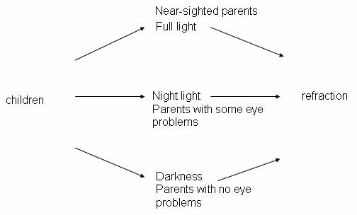
The initial steps of Investigation 1.3.1 should start feeling fairly routine for students by this point. You might consider asking them to complete up to a certain question before they come to class. It is also fun to ask them whether or not they wear glasses and if they remember the type of lighting they had as a child. The key point is of course the distinction between association and causation and through class discussion students should be able to suggest some reasonable confounding variables. Where to be picky is to make sure that their confounding variable has a clear connection to the response (eye condition) and that there is the differentiation in this variable between the explanatory variable groups (type of lighting). Students tend to describe the connection to the response but not to the explanatory variable. It can be helpful to ask students to think of confounding as an alternative explanation, as opposed to a cause/effect explanation, for the association between the variables. You might consider having them practice drawing an experimental design schematic (formally introduced later in the course), along with matching the different confounding variable outcomes with the different explanatory variable outcomes. For example:
The practice problems at the end of this investigation are a little more subtle than earlier ones and it will be important to discuss them in class and ensure that students understand the two things they need to discuss to identify a variable as potentially confounding (its connection to both the explanatory and the response variable).
In Investigation 1.3.2, we have chosen to treat Simpson’s Paradox as another confounding variable situation. This investigation goes into the mathematical formula as another way to illustrate the source of the paradox (the imbalance in where the women applied and an imbalance in the acceptance rates of the two programs). You might also consider showing them a visual illustration such as:
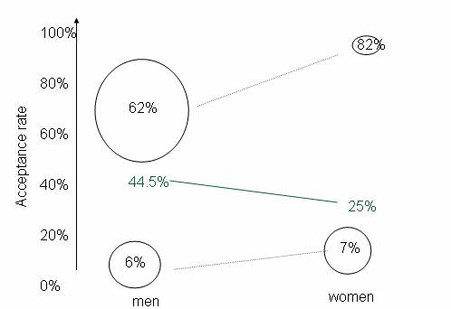
where the size of the circles are intended to convey the sample sizes in each category and thus their overall “weight” in the overall calculation.
Students will probably struggle a bit with (i) and (j) but hopefully can see the relationships if taken one step at a time.
Practice problem 1.3.3 will help them see the paradox arising in a different setting. Even when they see and pretty much understand what’s going on, students often struggle to provide a complete explanation of the cause of the apparent paradox. A very good follow-up question is to ask them to construct hypothetical data for which Simpson’s Paradox occurs as in Practice problem 1.3.4.
It will be important to convey to students exactly what “skills” and “concepts” you want them to take away from this investigation. If you want to focus on the “weighted average” idea (which has some nice reoccurrences later in the course), students will probably need a bit more practice. In summarizing these investigations with students, we are hoping they have motivated the need for more careful types of study designs that would avoid the confounding issues. Students often have an intuitive understanding of “random assignment” but this will be developed more formally in the next section.
Section 1.4: Designing Experiments
Timing/Materials: This section will probably take approximately 45-50 minutes. Some of the simulations could be assigned to out of class. You will need index cards for the tactile simulation and access to an internet browser. Students have access to all of the data files and java applets page here and through the CD that comes with the text. Much of Investigation 1.4.1 will probably be familiar to them and we recommend going through it with students rather quickly.
In Investigation 1.4.1, students see yet another example of
the limitations of an observational study and are usually very good at
identifying potential confounding variables.
It’s fun (and motivating) to ask students if they know whether their
institution has a foreign language requirement and what might be the reasons
for that requirement. Deciding whether
foreign language study directly increases verbal ability (as posited by many
deans) leads into the idea of an experiment and most students appear to have
heard these terms, including placebo, before.
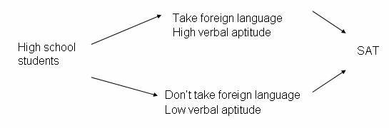
You may also wish to
discuss with them the schematic for the original observational study and the
potential “verbal aptitude” confounding variable:
In Investigation 1.4.2, we strive to help students see the benefits of randomization. We have students begin with a hands-on simulation of the randomization process. We feel this engages the students and gives them a concrete model of the process. We encourage you to have the students come to the board to collectively create the dotplot of their results in (d). Students could conduct the randomization outside of class and bring in their results but we feel this concept is important enough that you may prefer to do so in class. Students then transition to an applet to perform the randomization process many, many more times. Hopefully the prior hands-on simulation and the graphics of the applet will help them connect to the computer simulation (and reinforce that they are mimicking the randomization process used by the researchers). Nevertheless, be aware that some students click through the applet quickly without stopping to think about what it reveals. You might want to ask a question like “Where would an outcome show up in the dotplot if a repetition was unlucky and did not balance out the heights between the groups?” They should be able to work through the applet questions fairly quickly and then you will want to emphasize that randomization “evens out” other lurking or extraneous variables between the groups, typically not even recorded or seen by the researchers, as illustrated by the “gene” and “x” variables in the applet. It is important to emphasize to students that while we often throw around the word “random” in everyday usage, achieving true “statistical randomness” takes some effort and should not be short-circuited.
Practice problem 1.4.1 tests their understanding of what constitutes an experiment and we prefer to focus on the imposition of the explanatory variable (which was not done here). Practice problem 1.4.2 asks them to compare other types of randomization schemes and Practice problem 1.4.3 highlights that experimental studies are not always feasible. These questions are especially good for generating class discussion (rather than to suggest strict correct and incorrect solutions).
Investigation 1.4.3 is listed as optional or may be presented briefly. It continues to use the applet to have students think about the concept of “blocking.” We have chosen to discuss a rather informal use of “blocking” in that students are first manually splitting subjects into homogenous groups. The applet conveys the idea that if you actively balance out factors such as gender between the two groups, that will ensure further balance between the groups on some other variables as well (those related to gender, like height). We chose not to emphasize this concept strongly but did want students to think about the advantages (and disadvantages) of carrying out the experimental design on a more homogeneous group of subjects.
At this point in the course, you might also consider assigning a data collection project where students work with categorical variables and consider both observational and experimental studies. An example set of project assignments is posted here.
Section 1.5: Assessing Statistical Significance
Timing/Materials: With some review of the idea of confounding variables at the beginning, this section takes approximately 60 minutes. One timing consideration is that we have students do a second tactile simulation. This simulation is very similar to that in Section 1.4 but here focuses on the response instead of the explanatory variable. Still, you may want to make sure these simulations occur on different days. We do see value in having students do both as they too easily forget what the randomization in the process is all about (and how we can make decisions in the presence of randomness). This simulation also ties closely to an applet and helps transition students to the concept of a p-value. You will need pre-sorted playing cards or index cards and access to an internet browser. We pre-sort the playing cards into packets of 24, with 11 black ones (clubs/spaces) representing successes and 13 red ones (hearts/diamonds) representing failures, but you could also use index cards and have students mark the successes and failures themselves.
The goal in this section is to see the entire statistical process, from consideration of study design, to numerical and graphical summaries, to statistical inference. Students learn about the idea of a p-value by simulating a randomization test. One way to introduce this section is to say that even after we’ve used randomization to eliminate confounding variables as potential explanations for an association between the explanatory and response variables, another explanation still exists: maybe the observed association is simply the result of random variation. Fortunately, we can study the randomization process to determine how likely this is. While in the previous section we focused on how randomization evens out the effects of other extraneous variables, here the focus is on how large the difference in the response variable might be just due to chance alone, if there were really no difference between the two explanatory groups. You will want to greatly emphasize the question of how to determine whether a difference is “statistically significant.” Try to draw students to think about “what would happen by chance,” even before the simulation, as a way to answer this question (around question (f)). At some point (beginning of class, around question (f), end of class) you may even want to detour to another example to illustrate the logical thinking of statistical significance. One demonstration that we have found effective is to have a student volunteer roll a pair of dice that look normal but are actually rigged to roll only sums of seven and eleven (e.g., unclesgames.com, other sources). Students realize after a few rolls that the outcomes are too surprising to have happened by chance alone for normal dice and thus provide compelling evidence that there is something fishy about the dice. It is important for students to think of the randomization distribution as a “what if” exploration to help them analyze the experimental results actually obtained.
For part (i) of Investigation 1.5.1, we have students create a dotplot on the board, with each student placing five dots (one for each repetition of the randomization process) on the plot. You can also have students turn in their results for you to compile between classes or have them list their results to you orally (or as you walk around the room) while you (or a student assistant) type them into Minitab or place them on the board yourself. In part (s), it’s instructive to ask several students to report what they obtain for the empirical p-value, because students should see that while these estimates differ from student to student, they are actually quite similar.
The data described in Investigation 1.5.1 have been slightly altered. In the actual study, 11 observers were assigned to Group A and 12 to Group B, however we preferred that these column totals were not the same as the row totals. Students should find the initial questions very straight forward and again you could ask them to complete some of this background work prior to the class meeting.
Some notes on the applet:
- holding the mouse over the deck of cards reveals the composition of the deck (students should note the 13 red and the 11 black cards).
- with 1000 repetitions, when you “show tallies” the values tend to crash a bit, but students should be able to parse them out.
- the “Difference in Proportion” button is to help students
see the transition between this distribution and the distribution of ![]() A –
A – ![]() B that
they will work with later but it may not be worth addressing at this point in
the course.
B that
they will work with later but it may not be worth addressing at this point in
the course.
- we encourage you to continually refer to the visual image of the empirical randomization distribution given by the applet when interpreting p-values.
One distinction in terminology that you may want to highlight for students is that the term “randomization distribution” refers to all possible randomizations, while the phrase “empirical randomization distribution” means the approximation to the randomization distribution, generated by a simulation that repeats the randomization process a large number of times.
There are some important points for students to be comfortable with in the discussion on p. 50. In particular, we want students to realize throughout the course how the p-value presents a measure of the strength of evidence along a continuous scale. You might tell students to think of this as a grayscale and not just black/white. You will also want to emphasis that the p-value measures how often research results at least this extreme would occur by chance if there was no true difference between the experimental groups. You might also want to remind students that the terminology introduced in this investigation will be used throughout the rest of the course.
Section 1.6: Probability and Counting Methods
Timing/Materials: This section, consisting of two investigations, should take approximately 65 minutes, but could be much less if your students are already familiar with combinations. You may also choose to supplement with some other probability applications and/or discussion of lotteries. An applet is used in both investigations, and you may want to use Excel in Investigation 1.6.2.
At this point, quantitatively inclined students are often chomping at the bit for a more analytic approach for determining “exact p-values” that circumvents the need for the approximating simulations. Investigation 1.6.1 introduces them to the idea of probability as the long-run relative frequency of an outcome in a rather silly, but memorable, “application.” We apologize for the context, but students do tend to remember it and the investigation is closely tied to a java applet that graphs the behavior of the empirical probability over the number of repetitions. It will be important to have longer discussions on what the applet’s pictures represent (either as a class or a writing assignment). This investigation also introduces the idea, and parallel interpretation, of expected value. We emphasize two aspects of interpreting expected value: long-run and average; some students tend to ignore the “average” part. You will especially want to recap the idea of a random variable with your students.
At this point you may choose to introduce some other interpretations of probability, e.g., subjective probability, to introduce them to the diversity of uses of the term. Also, while the calculations in this course often make use of the equal probability of outcomes from the randomization, you might want to caution them to not always assume outcomes are equally likely. The following transcript from a Nightline broadcast a few years about may help bring home the point:

In Investigation 1.6.2, students use this basic probability knowledge to calculate a probability using combinations, emphasizing the distinction between an empirical and an exact probability. You may want to show your students how to do these combination calculations on their calculator as well as in Excel. We often also advise students that we are more interested in their ability to set up the calculation (e.g., on an exam). We also strive to keep the “statistical motivation” of these calculations in mind – how often do experimental results as extreme as this happen “by chance.” In using the Two-way Table Simulation applet, the default calculated p-value is always calculated as the probability of the observed number of successes in Group A and below. To change this, using the version of the applet on the web (not the CD), first press the “<=” button to toggle to “>=”. Then the empirical p-value button will be found by counting the number of successes in Group A observed or higher. In this problem, we ask students to find “as many successes” in the coated suture group, you may want to motivate this direction with your students.
Section 1.7: Fisher’s
Exact Test
Timing: This section should take about 100 minutes. You may also wish to provide more practice carrying out Fisher’s Exact Test and discussing the overall statistical process. In Investigation 1.7.1, students are asked to create a segmented bar graph and calculate p-values (meaning technology is helpful but not essential). They are also asked to compare back to their simulation results in Investigation 1.5.1.
Investigation 1.7.1 brings the statistical analysis full circle by formally introducing the hypergeometric probabilities to calculate p-values for two-way tables and pulling together the ideas of the previous two sections. It first continues the analysis of the “Friendly Observers” study, for which students have only approximated the p-value so far, and asks them to calculate the exact p-value now that they are knowledgeable of combinations (and the addition rule for probabilities). The questions step them through constructing hypergeometric probabilities. You may want to help them through this as a class and then emphasize the structure of the calculations. It is also worth showing them that the same calculation can be set up several different ways and arrive at the same p-value (as long as they are consistent), e.g., top of p. 68. Many students struggle with this, but it is worth helping them to understand, because then they do not have to worry about which category to consider “success” or “failure.” Students are then asked to turn the calculations over to Minitab. We hope students will soon become comfortable using Minitab to calculate these probabilities and we try not to spend too long on the combinations calculations. We show several ways to arrive at the calculations so that they may find the method they are most comfortable with. You can also use Minitab or other software to show them lots of graphs of the hypergeometric distribution for different parameter values. The investigation also reminds them of the idea of expected value and how it may be calculated. Question (s) and (t) are important for helping students use the complement rule with integer values to calculate (upper-tail) p-values in Minitab. This idea will occur quite frequently in the course, and many students struggle with it, so it is important to get them used to it quickly. Beginning with question (u), Investigation 1.7.1 transitions into focusing on the effect of sample size on the p-value. This gives students additional practice while making a very important statistical point that will recur throughout the course.
Investigation 1.7.2 gives them additional practice with Fisher’s Exact Test but also brings up the debate of what the p-value really means with observational data. We like to tell students that with observational studies, a very small p-value can essentially eliminate random variation as an explanation (for an observed association between explanatory and response variables), but the possibility of confounding variables cannot be ruled out.
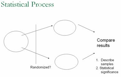
Summary
Students need to be strongly encouraged to read the Chapter Summary and the Technology Summary. If the classroom environment is more “discovery-oriented,” students will need to carefully organize their notes. You should remind them that this course will be rather “cyclic” in that these ideas will return and be built upon in later chapters. You might also consider showing students a graphic of the overall statistical process and how the ideas they have learned so far fit in, e.g.:
With these students, we have had good luck asking them to submit potential exam questions as part of the review process.