INVESTIGATING STATISTICAL CONCEPTS, APPLICATIONS, AND METHODS

NOTES FOR INSTRUCTORS

Chapter 1 Chapter 2 Chapter 3 Chapter 4 Chapter 5 Chapter 6

General Notes:

We envision the materials as being very flexible in how they are used. You may choose to lead students through many of the investigations together as a class, but we also encourage you to give students time to work through some questions on their own (or better in pairs) and then debrief with the students afterwards. If you do have students work through investigations largely on their own, it’s very important to conduct a wrap-up discussion at the end of class, and/or at the beginning of the next class, in which you make clear what the “morals” of the investigations were.  In other words, summarize for students what they were supposed to have learned through the investigations and what they are responsible for knowing, making sure they are reading the additional exposition in the text as well.  These wrap-up discussion times are also ideal for inviting students’ questions, because they will have wrestled with the ideas enough to know what the issues are and where their understanding is shaky. You may wish to collect students’ answers to just a few of the questions in an investigation to read over and give feedback before the next class session. The practice problems are intended to provide students with basic review and practice of the most recent ideas between class periods. This will help structure their time outside of class, and provide a way for you and the students to informally assess their understanding and provide feedback. You may choose to collect and grade these as homework problems or use them more to motivate initial discussion in the next class period. You can also consider including a “participation” component in your syllabus to include effort if your evaluation will be more informal. Solutions have been posted online. They are password protected giving the instructor the option of giving students direct access or not. These problems also work well in a course management system such as Blackboard or WebCT for more automatic submission and feedback.

You may also wish to supplement some of the material in the book, e.g., bringing in recent news articles for discussion, or assigning data collection project assignments. We think students will find the ISCAM investigations interesting and motivating, but there will also be time to share other examples as well. Some students prefer to read through examples worked out in detail and we have provided at least one such example at the end of each chapter. If you do bring in your own material, we do caution you to try to remain consistent with the text in terminology, notation, and sequencing of ideas. Some of this material and sequencing may be new to you as the instructor and may take a while to get used to. Keep in mind that the material you think is usually introduced at different points in the course will be coming eventually.

We have written the materials assuming students will have easy access to a computer, and we make increasing use of technology as the course progresses. We have taught the course with daily access to a computer lab, but believe it will also work with less frequent visits to a computer lab and/or more instructor demonstrations (using a computer projection system). If the students do not have frequent access to computers during class, you may wish to assign more of the computer work to take place outside of class. We do provide detailed instructions for all of the computer work (Minitab, Excel, java applets), but you may still want to encourage students to work together. We have also assumed use of Minitab 14 but at the Minitab Hints page will try to outline where you will have to make adjustments to use Minitab 13 as well as suggestions for making additional use of Minitab 14’s new capabilities (e.g., automatic graph updating). Even with heavy use of computers, it is also nice to have some days where you focus less on the computers to give students a chance to ask questions on the larger concepts in the material and even work a few calculations “by hand.” Student will use a calculator on a daily basis as well.

The following elements will be found in each chapter:

Investigations: These are intended to be “covered” during the lecture period, either as note pages for the class to complete together or as worksheets for students to work on individually or in pairs. Often, a section can correspond to one 50-60 minute class period.

Practice Problems: These are intended as quick reviews of the basic ideas and terminology of the previous investigation(s) and can often be assigned between class periods. They can be located by the small blue page bar.

Explorations: These are a bit more open-ended explorations of additional statistical content (e.g., uncovering mathematical properties of odds ratio vs. relative risk, deeper consideration of sampling plans, properties of confidence interval methods based on different degrees of freedom). The explorations typically involve heavy software usage and work well as “lab assignments” that students can complete inside or outside of class.

Examples: Each chapter contains at least one example worked out for students to see the solution approach in detail. The pages on which they occur have a long blue edge bar.

Chapter Summary and Technology Summary: These provide a review list of the main concepts covered in the chapter as well as the basic computer commands that will be used in subsequent chapters.

Exercises: At the end of each chapter is a large set of exercises covering material from throughout the chapter. The exercises include a combination of conceptual questions, application exercises, and mathematical explorations.

References: A list of the study references for all investigations, practice problems and exercises appears at the end of each chapter.

In aiming to make the materials easy to navigate, we have adopting the following numbering scheme:

Section x.y refers to the y^th section in chapter x

Investigation x.y.z refers to the z^th investigation of the y^th section in chapter x

Practice Problem x.y.z refers to the z^th problem in Chapter x, Section y

Exploration a.b refers to an Exploration in Chapter a, Section b.

If multiple explorations occurs in a section, they are given a third number as well.

Example c.d is the d^th example of the c^th chapter and is located at the end of the chapter (before the exercises).

Prologue: Traffic Deaths in Connecticut

Timing: Taking roll, explaining the syllabus, telling students a bit about what the course would be like, and then going through prologue together (giving them a chance to think about the issues first) took about 50 minutes. You might consider asking them to read some of the background information and even answer the first few questions in Investigation 1.1.1 before arriving to the next class period.

The goal of the Prologue is to introduce them to some key concepts and ways of thinking statistically that will hopefully recur throughout the course. It’s also important to get them used to thinking about the ideas of their own first before you discuss them in class. Students can usually provide very good answers to these questions and you should summarize by reminding them how important it is to make “fair” comparisons.

Section 1.1: Summarizing Categorical Data

Timing: Answering additional questions (e.g., explaining the different elements of the text) and having them work through Investigation 1.1.1 took about 50 minutes. Students are asked to make a graph in Excel but that can be easily moved to outside of class (perhaps after an instructor demonstration).

Some additional information about the study in Investigation 1.1.1:

- You might consider showing students a copy of the journal article to demonstrate its authenticity. You can also find some links on the web to the ensuing court case. A recent one may still be here or here.

- In May, 2000: eight persons who had worked at the same microwave-popcorn production plant were reported to have bronchiolitis obliterans. No recognized case was identified in the plant. Therefore, they medically evaluated current employees and assessed their occupational exposure in Nov. 2000.

- They used a combination of questionnaires and spirometric testing. They also compared information to the National Health NE Survey

- The results here focus on the results of the spirometric testing: 31 people had abnormal results, 10 with low FVC (forced vital capacity) values, 11 with airway obstruction, and 10 with both airway obstruction and low FVC.

- Diacetyl is the predominant ketone in artificial butter flavoring and was used as a marker of organic-chemic exposure

- They tested air samples and dust samples from various areas in the plant. These areas included

Plain-popcorn packaging line, bag-printing areas, warehouse, offices, outside

Quality control or maintenance

Microwave-popcorn packaging lines

Mixing room

The first group is considered “non-production” so lower exposure but they also looked at how long employees had worked in different areas to classify them as “high exposure” and “low exposure.”

In (e), get students to tell you about their description of the graph – solicit descriptions from several people. Make sure the descriptions are in context and include the comparison. You will probably be able to tell them that all the responses were good and that one distinction between statistics and other subjects is that there can be multiple correct answers. When students offer suggestions about reasons for the difference in the groups, make sure they discuss a factor that differs between the two groups. So saying “other health issues” isn’t enough, but a better answer is saying that those who worked in certain areas of the plant may have different SES status than those who work in the production areas of the plant or that they may be more likely to live in the country which has different air quality, etc. Really get them to suggest the need for comparison, either to people outside the plant or to people in different areas of the plant. Also build up the idea of not just comparing the counts but converting to proportions first.

In (i), you might also want to ask students to calculate the relative risk for (h) and see that it turns out different than for (c), even though the difference in proportions is the same.

In (k), we encourage you to go through the odds ratio calculations. You might consider asking a student in the class to define odds, but you need to build up the odds ratio slowly and always encourage them to interpret the calculation correctly, because precisely interpreting the odds ratio is tricky for most students and requires much practice.

Page 7: It’s important that students get a chance to practice with the vocabulary soon as it is not as easily mastered as they may initially think. You especially need to watch that they state variables as variables. Too often they will want to say “lung cancer” instead of describing the entire variable (“whether or the person has lung cancer”). Or they will slip into summaries like “the number with lung cancer.” Or they will combine the variables and the observational units: “those with lung cancer.” We strongly recommend trying to get them to think of the variable as the question asked of each observational unit.

The practice problems are intended to get students to work more with variables. Much of the terminology will be unfamiliar to them or they will have other “day-to-day” definitions so it is important to “immerse” them into the vocabulary and allow them to practice it often. We suggest beginning the next class by discussing these problems, especially 1.1f and 1.1.2. We highly encourage you to either collect students’ work on the practice problems (reading through and commenting on their responses) and/or to briefly discuss them at the beginning of the next class period. We envision these as being a more informal, thought provoking, self-check form of assessment.

We have included “section summaries” at the end of the sections. This is a good place to ask students if they have questions on the material so far. You might also consider adapting these into bullet points to recap the previous class period at the start of the next class period. You may want to remind students occasionally that they should read all of the study conclusion, discussion, and summary sections carefully; some students get in the habit of working through the investigations by answering questions but do not “slow down” enough to read through and understand the accompanying exposition.

Section 1.2: Analyzing Categorical Data

Timing: Students were able to complete Investigation 1.2.1 and 1.2.2 in approximately 60 minutes. We did Investigation 1.2.1 mostly together but then students worked on Investigation 1.2.2 in pairs. You may wish to have students complete some of the Excel work outside of class (including for Investigation 1.2.1 prior to coming to class). Exploration 1.2 makes heavy use of Excel but no other technology.

Investigation 1.2.1 gives students immediate practice in applying the terminology of Section 1.1. We strongly encourage you to allow the students to work through these questions, at least through (j), on their own first. Question (c) asks students to use Excel, but again they could do that outside of class or you could demonstrate it for them. Students will struggle and you need to visit them often to make sure they are getting the answers correct (e.g., how they state the variables, whether they see “amount of smoking” as categorical, and calculation of the odds-ratios). The odds-ratios questions are asked to encourage them to treat having lung cancer as a success and putting the non-smokers odds in the denominator. This ensures the odds-ratio is greater than one and treats the non-smokers as the reference group to compare to. The main criticism we expect to hear about in (j) is age but even after the odds-ratios were “adjusted” for age there could be other differences between the groups again, e.g., socio-economic status, diet, exercise that are related to both smoking status and occurrence of lung cancer.

Question (l) is a subtle point but important for students to think about. The point here is that this proportion is not a reasonable estimate because the experimenters fixed the number of lung cancer and control patients by design (i.e., a case-control study). In this text, we tend to distinguish between the types of study (case-control, cohort, cross-classification) and the type of design (retrospective, prospective). These are not clear distinctions and you may not wish to spend too long on them. It is much more important for students to distinguish between observational studies and experiments, but also always considering the implications of the study design on the final interpretations of the results. Questions (m) and (n), about when we can draw cause/effect conclusions and when we can generalize results to larger population, are important ones that will arise throughout the course, so it’s worth drawing students’ attention to them. In particular, we want students to get into the habit of seeing these as two distinct questions, answered based on different criteria, to always be asked when summarizing the conclusions of a study.

Investigation 1.2.2 provides students with more practice and gets them to again think in terms of association. They should be able to tell you some advantages to the prospective design over the retrospective design (e.g., not relying on memory, seeing what develops instead of taking people who are already sick). However this does not take into account any of the other possible confounding variables or that they only selected healthy, white men initially. You may want to pre-create the Excel worksheet for them and then have them open it and start from there.

The Excel Exploration can be done inside or outside of class. I had students finish it in pairs outside of class and then turn in a report of their results. They should see that the odds-ratio and the relative risk are similar when the baseline risk is small and that they can be very different from 1 even for the same difference in proportions. This is also the first time they really see that the OR and RR are equal to one when the difference in proportions is zero. We encourage you to have them view the updating segmented bar graph throughout these calculations to also see the changes visually. This exploration is essentially playing with formulas but allows them to come to a deeper understanding of the formulas, how to express them, and hopefully how they are related. Some issues you might want to ask them about afterwards (in class or in a written report) include:

- when will RR and OR be similar in value (you can even lead a discussion of the mathematical relationship OR = RR(1-p₂)/(1-p₁) )

- when are RR and OR more useful values to look at than the difference in proportions (primarily when the success proportions are very small or very large)

- when will RR and OR be equal to 1 and what does that imply about the relationship between the variables/the difference in proportions

These comparisons should fall out if they follow the structure of the examples and what changed with each table. You also need to decide how much of the Excel output you want them to turn in.

As you summarize these first 3 investigations you might even want to warn them that they won't see RR and OR too much for a while but the other big lessons they should be taking from this early material is the importance of the study design and always using graphical and numerical summaries as they explore the data. Students should also be getting the idea that statistics matters and that statistics is important for investigating important issues.

Additionally you can highlight the three studies they have seen so far (Popcorn, Wynder and Graham, Hammond and Horn) and compare and contrast them. For example:

Popcorn and lung disease	Wynder and Graham	Hammond and Horn
Defined subjects as high/low exposure, classified airway obstruction	Found subjects with and without lung cancer, classified smoking status (case-control, retrospective)	Followed subjects, found level of smoking, whether died of lung cancer (cross-classified, prospective)
Meaningful to examine proportion with airway obstruction	Not meaningful to examine proportion with lung cancer	Meaningful to examine proportion who died of lung cancer and proportion of smokers
Similar number in each explanatory variable group	Similar number in each response variable group
May not be representative	Controlled interviewer behavior	Not much control (22,000 ACS volunteers)

You may wish to summarize why the “invariance” of odds ratios helps to explain why they are preferred in many situations instead of the easy to interpret relative risk. For example, with odds ratio, it does not matter which category is considered the success.

Section 1.3 Confounding

Timing: This section will probably take approximately 45-50 minutes. You may choose to do more leading in this section in the interest of time. No technology is used.

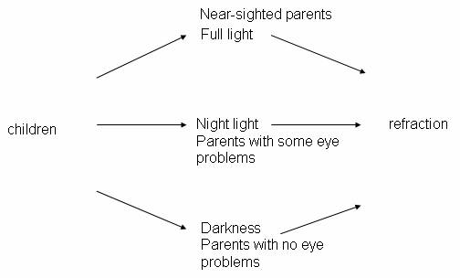
The initial steps of Investigation 1.3.1 should start feeling fairly routine for students by this point. You might consider asking them to complete up to a certain question before they come to class. It is also fun to ask them whether or not they wear glasses and if they remember the type of lighting they had as a child. The key point is of course the distinction between association and causation and through class discussion students should be able to suggest some reasonable confounding variables. Where to be picky is to make sure that their confounding variable has a clear connection to the response (eye condition) and that there is the differentiation in this variable between the explanatory variable groups (type of lighting). Students tend to describe the connection to the response but not to the explanatory variable. It can be helpful to ask students to think of confounding as an alternative explanation, as opposed to a cause/effect explanation, for the association between the variables. You might consider having them practice drawing an experimental design schematic (formally introduced later in the course), along with matching the different confounding variable outcomes with the different explanatory variable outcomes. For example:

The practice problems at the end of this investigation are a little more subtle than earlier ones and it will be important to discuss them in class and ensure that students understand the two things they need to discuss to identify a variable as potentially confounding (its connection to both the explanatory and the response variable).

In Investigation 1.3.2, we have chosen to treat Simpson’s Paradox as another confounding variable situation. This investigation goes into the mathematical formula as another way to illustrate the source of the paradox (the imbalance in where the women applied and an imbalance in the acceptance rates of the two programs). You might also consider showing them a visual illustration such as:

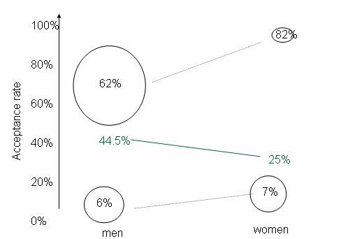
where the size of the circles are intended to convey the sample sizes in each category and thus their overall “weight” in the overall calculation.

Students will probably struggle a bit with (i) and (j) but hopefully can see the relationships if taken one step at a time.

Practice problem 1.3.3 will help them see the paradox arising in a different setting. Even when they see and pretty much understand what’s going on, students often struggle to provide a complete explanation of the cause of the apparent paradox. A very good follow-up question is to ask them to construct hypothetical data for which Simpson’s Paradox occurs as in Practice problem 1.3.4.

It will be important to convey to students exactly what “skills” and “concepts” you want them to take away from this investigation. If you want to focus on the “weighted average” idea (which has some nice reoccurrences later in the course), students will probably need a bit more practice. In summarizing these investigations with students, we are hoping they have motivated the need for more careful types of study designs that would avoid the confounding issues. Students often have an intuitive understanding of “random assignment” but this will be developed more formally in the next section.

Section 1.4: Designing Experiments

Timing/Materials: This section will probably take approximately 45-50 minutes. Some of the simulations could be assigned to out of class. You will need index cards for the tactile simulation and access to an internet browser. Students have access to all of the data files and java applets page here and through the CD that comes with the text. Much of Investigation 1.4.1 will probably be familiar to them and we recommend going through it with students rather quickly.

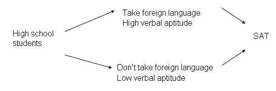
In Investigation 1.4.1, students see yet another example of the limitations of an observational study and are usually very good at identifying potential confounding variables. It’s fun (and motivating) to ask students if they know whether their institution has a foreign language requirement and what might be the reasons for that requirement. Deciding whether foreign language study directly increases verbal ability (as posited by many deans) leads into the idea of an experiment and most students appear to have heard these terms, including placebo, before.

You may also wish to discuss with them the schematic for the original observational study and the potential “verbal aptitude” confounding variable:

In Investigation 1.4.2, we strive to help students see the benefits of randomization. We have students begin with a hands-on simulation of the randomization process. We feel this engages the students and gives them a concrete model of the process. We encourage you to have the students come to the board to collectively create the dotplot of their results in (d). Students could conduct the randomization outside of class and bring in their results but we feel this concept is important enough that you may prefer to do so in class. Students then transition to an applet to perform the randomization process many, many more times. Hopefully the prior hands-on simulation and the graphics of the applet will help them connect to the computer simulation (and reinforce that they are mimicking the randomization process used by the researchers). Nevertheless, be aware that some students click through the applet quickly without stopping to think about what it reveals. You might want to ask a question like “Where would an outcome show up in the dotplot if a repetition was unlucky and did not balance out the heights between the groups?” They should be able to work through the applet questions fairly quickly and then you will want to emphasize that randomization “evens out” other lurking or extraneous variables between the groups, typically not even recorded or seen by the researchers, as illustrated by the “gene” and “x” variables in the applet. It is important to emphasize to students that while we often throw around the word “random” in everyday usage, achieving true “statistical randomness” takes some effort and should not be short-circuited.

Practice problem 1.4.1 tests their understanding of what constitutes an experiment and we prefer to focus on the imposition of the explanatory variable (which was not done here). Practice problem 1.4.2 asks them to compare other types of randomization schemes and Practice problem 1.4.3 highlights that experimental studies are not always feasible. These questions are especially good for generating class discussion (rather than to suggest strict correct and incorrect solutions).

Investigation 1.4.3 is listed as optional or may be presented briefly. It continues to use the applet to have students think about the concept of “blocking.” We have chosen to discuss a rather informal use of “blocking” in that students are first manually splitting subjects into homogenous groups. The applet conveys the idea that if you actively balance out factors such as gender between the two groups, that will ensure further balance between the groups on some other variables as well (those related to gender, like height). We chose not to emphasize this concept strongly but did want students to think about the advantages (and disadvantages) of carrying out the experimental design on a more homogeneous group of subjects.

At this point in the course, you might also consider assigning a data collection project where students work with categorical variables and consider both observational and experimental studies. An example set of project assignments is posted here.

Section 1.5: Assessing Statistical Significance

Timing/Materials: With some review of the idea of confounding variables at the beginning, this section takes approximately 60 minutes. One timing consideration is that we have students do a second tactile simulation. This simulation is very similar to that in Section 1.4 but here focuses on the response instead of the explanatory variable. Still, you may want to make sure these simulations occur on different days. We do see value in having students do both as they too easily forget what the randomization in the process is all about (and how we can make decisions in the presence of randomness). This simulation also ties closely to an applet and helps transition students to the concept of a p-value. You will need pre-sorted playing cards or index cards and access to an internet browser. We pre-sort the playing cards into packets of 24, with 11 black ones (clubs/spades) representing successes and 13 black ones (hearts/diamonds)) representing failures, but you could also use index cards and have students mark the successes and failures themselves.

The goal in this section is to see the entire statistical process, from consideration of study design, to numerical and graphical summaries, to statistical inference. Students learn about the idea of a p-value by simulating a randomization test. One way to introduce this section is to say that even after we’ve used randomization to eliminate confounding variables as potential explanations for an association between the explanatory and response variables, another explanation still exists: maybe the observed association is simply the result of random variation. Fortunately, we can study the randomization process to determine how likely this is. While in the previous section we focused on how randomization evens out the effects of other extraneous variables, here the focus is on how large the difference in the response variable might be just due to chance alone, if there were really no difference between the two explanatory groups. You will want to greatly emphasize the question of how to determine whether a difference is “statistically significant.” Try to draw students to think about “what would happen by chance,” even before the simulation, as a way to answer this question (around question (f)). At some point (beginning of class, around question (f), end of class) you may even want to detour to another example to illustrate the logical thinking of statistical significance. One demonstration that we have found effective is to have a student volunteer roll a pair of dice that look normal but are actually rigged to roll only sums of seven and eleven (e.g., unclesgames.com, other sources).  Students realize after a few rolls that the outcomes are too surprising to have happened by chance alone for normal dice and thus provide compelling evidence that there is something fishy about the dice. It is important for students to think of the randomization distribution as a “what if” exploration to help them analyze the experimental results actually obtained.

For part (i) of Investigation 1.5.1, we have students create a dotplot on the board, with each student placing five dots (one for each repetition of the randomization process) on the plot. You can also have students turn in their results for you to compile between classes or have them list their results to you orally (or as you walk around the room) while you (or a student assistant) type them into Minitab or place them on the board yourself. In part (s), it’s instructive to ask several students to report what they obtain for the empirical p-value, because students should see that while these estimates differ from student to student, they are actually quite similar.

The data described in Investigation 1.5.1 have been slightly altered. In the actual study, 11 observers were assigned to Group A and 12 to Group B, however we preferred that these column totals were not the same as the row totals. Students should find the initial questions very straight forward and again you could ask them to complete some of this background work prior to the class meeting.

Some notes on the applet:

- holding the mouse over the deck of cards reveals the composition of the deck (students should note the 13 red and the 11 black cards).

- with 1000 repetitions, when you “show tallies” the values tend to crash a bit, but students should be able to parse them out.

- the “Difference in Proportion” button is to help students see the transition between this distribution and the distribution of _A – _B that they will work with later but it may not be worth addressing at this point in the course.

- we encourage you to continually refer to the visual image of the empirical randomization distribution given by the applet when interpreting p-values.

One distinction in terminology that you may want to highlight for students is that the term “randomization distribution” refers to all possible randomizations, while the phrase “empirical randomization distribution” means the approximation to the randomization distribution, generated by a simulation that repeats the randomization process a large number of times.

There are some important points for students to be comfortable with in the discussion on p. 50. In particular, we want students to realize throughout the course how the p-value presents a measure of the strength of evidence along a continuous scale. You might tell students to think of this as a grayscale and not just black/white. You will also want to emphasis that the p-value measures how often research results at least this extreme would occur by chance if there was no true difference between the experimental groups. You might also want to remind students that the terminology introduced in this investigation will be used throughout the rest of the course.

Section 1.6: Probability and Counting Methods

Timing/Materials: This section, consisting of two investigations, should take approximately 65 minutes, but could be much less if your students are already familiar with combinations. You may also choose to supplement with some other probability applications and/or discussion of lotteries. An applet is used in both investigations, and you may want to use Excel in Investigation 1.6.2.

At this point, quantitatively inclined students are often chomping at the bit for a more analytic approach for determining “exact p-values” that circumvents the need for the approximating simulations. Investigation 1.6.1 introduces them to the idea of probability as the long-run relative frequency of an outcome in a rather silly, but memorable, “application.” We apologize for the context, but students do tend to remember it and the investigation is closely tied to a java applet that graphs the behavior of the empirical probability over the number of repetitions. It will be important to have longer discussions on what the applet’s pictures represent (either as a class or a writing assignment). This investigation also introduces the idea, and parallel interpretation, of expected value. We emphasize two aspects of interpreting expected value: long-run and average; some students tend to ignore the “average” part. You will especially want to recap the idea of a random variable with your students.

At this point you may choose to introduce some other interpretations of probability, e.g., subjective probability, to introduce them to the diversity of uses of the term. Also, while the calculations in this course often make use of the equal probability of outcomes from the randomization, you might want to caution them to not always assume outcomes are equally likely. The following transcript from a Nightline broadcast a few years about may help bring home the point:

In Investigation 1.6.2, students use this basic probability knowledge to calculate a probability using combinations, emphasizing the distinction between an empirical and an exact probability. You may want to show your students how to do these combination calculations on their calculator as well as in Excel. We often also advise students that we are more interested in their ability to set up the calculation (e.g., on an exam). We also strive to keep the “statistical motivation” of these calculations in mind – how often do experimental results as extreme as this happen “by chance.” In using the Two-way Table Simulation applet, the default calculated p-value is always calculated as the probability of the observed number of successes in Group A and below. To change this, using the version of the applet on the web (not the CD), first press the “<=” button to toggle to “>=”. Then the empirical p-value button will be found by counting the number of successes in Group A observed or higher. In this problem, we ask students to find “as many successes” in the coated suture group, you may want to motivate this direction with your students.

Section 1.7: Fisher’s Exact Test

Timing: This section should take about 100 minutes. You may also wish to provide more practice carrying out Fisher’s Exact Test and discussing the overall statistical process. In Investigation 1.7.1, students are asked to create a segmented bar graph and calculate p-values (meaning technology is helpful but not essential). They are also asked to compare back to their simulation results in Investigation 1.5.1.

Investigation 1.7.1 brings the statistical analysis full circle by formally introducing the hypergeometric probabilities to calculate p-values for two-way tables and pulling together the ideas of the previous two sections. It first continues the analysis of the “Friendly Observers” study, for which students have only approximated the p-value so far, and asks them to calculate the exact p-value now that they are knowledgeable of combinations (and the addition rule for probabilities). The questions step them through constructing hypergeometric probabilities. You may want to help them through this as a class and then emphasize the structure of the calculations. It is also worth showing them that the same calculation can be set up several different ways and arrive at the same p-value (as long as they are consistent), e.g., top of p. 68. Many students struggle with this, but it is worth helping them to understand, because then they do not have to worry about which category to consider “success” or “failure.” Students are then asked to turn the calculations over to Minitab. We hope students will soon become comfortable using Minitab to calculate these probabilities and we try not to spend too long on the combinations calculations. We show several ways to arrive at the calculations so that they may find the method they are most comfortable with. You can also use Minitab or other software to show them lots of graphs of the hypergeometric distribution for different parameter values. The investigation also reminds them of the idea of expected value and how it may be calculated. Question (s) and (t) are important for helping students use the complement rule with integer values to calculate (upper-tail) p-values in Minitab. This idea will occur quite frequently in the course, and many students struggle with it, so it is important to get them used to it quickly. Beginning with question (u), Investigation 1.7.1 transitions into focusing on the effect of sample size on the p-value. This gives students additional practice while making a very important statistical point that will recur throughout the course.

Investigation 1.7.2 gives them additional practice with Fisher’s Exact Test but also brings up the debate of what the p-value really means with observational data. We like to tell students that with observational studies, a very small p-value can essentially eliminate random variation as an explanation (for an observed association between explanatory and response variables), but the possibility of confounding variables cannot be ruled out.

Summary

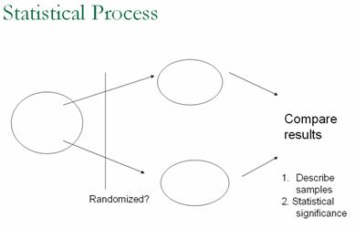
Students need to be strongly encouraged to read the Chapter Summary and the Technology Summary. If the classroom environment is more “discovery-oriented,” students will need to carefully organize their notes. You should remind them that this course will be rather “cyclic” in that these ideas will return and be built upon in later chapters. You might also consider showing students a graphic of the overall statistical process and how the ideas they have learned so far fit in, e.g.:

With these students, we have had good luck asking them to submit potential exam questions as part of the review process.

Chapter 2

This chapter parallels the previous chapter (considering of data collection issues, numerical and graphical summaries, and statistical inference from empirical p-values) but for quantitative variables instead of categorical variables. The themes of considering the study design and exploring the data are reiterated to remind students of their importance. Analyses for quantitative data are a bit more complicated than for categorical data, because no longer does one number suitably summarize a distribution by itself, and we also need to focus on aspects such as shape, center, and spread in describing these distributions. This also leads to heavier use of Minitab for analyzing data (e.g., constructing graphs and calculating numerical summaries) as well as for simulating randomization distributions. If your class does not meet regularly in a computer lab, you might want to consider having students work through the initial study questions of several investigations, saving up the Minitab analysis parts for when you can visit a computer lab. Or if you do not have much lab access, you could use computer projection to demonstrate the Minitab analyses. Keep in mind that there are a few menu differences if you are using Minitab 13 instead of Minitab 14 (see the powerpoint slides for Day 8 of Stat 212). One thing you will want to discuss with your students is the best way to save and import graphics for your computer setting. Some things we’ve used can be found here.

Section 2.1: Summarizing Quantitative Data

Timing/Materials:

This section covers graphical and numerical summaries for quantitative data, and these investigations will take several class sessions. Students will be using Minitab in Investigations 2.1.3 (oldfaithful.mtw), 2.1.5 (temps.mtw), and 2.1.6 (fan03.mtw,the ISCAM webpage also provides access to the most recent season’s data.). Instructions for replicating the output shown in Investigation 2.1.2 (CloudSeeding.mtw) are included as a Minitab Detour on p. 111. Excel is used in Investigation 2.1.7 (housing.xls). Investigations 2.1.1 and 2.1.2 together should take about 50-60 minutes. Investigations 2.1.3, 2.1.4, and 2.1.5 together should take another 60 minutes or so. Investigation 2.1.6 could take 40-50 minutes, and Investigation 2.1.7 could take 50-60 minutes. You might consider assigning Investigation 2.1.6 as a lab assignment that students work on in pairs and complete the “write-up” outside of class. Or you can expand on the instructions for Practice Problem 2.1.7 as the lab-writeup assignment. Investigation 2.1.7 explores the mathematical properties of least squares estimation in this univariate case and can be skipped or moved outside of class, perhaps as a “lab assignment.”

Investigation 2.1.1 is meant to provoke informal discussions of anticipating variable behavior. You may choose to wait until students have been introduced to histograms (in which case it could also serve to practice terminology such as skewness). One goal is to help students get used to having the variable along the horizontal axis with the vertical axis representing the frequencies of observational units. Furthermore, we want to build student intuition for how different variables might be expected to behave.

Students usually quickly identify graphs 1 and 6 as either the soda choice or the gender variable, the only categorical variables. Reasonable arguments can be made for either choice. In fact, we try to resist telling students there is one “right answer” (another habit of mind we want them to get into in this statistics class that some students may not be expecting, as well as that writing coherent explanations will be an expected skill in this class). We tell them we are more interested in their justification than their final choice, but that we see how well they support their answers and the consistency of their arguments. A clue could be given to remind students the name of the course these 35 students were taking. This often leads students to select graph 1 as the gender variable, assuming the second bar represents a smaller proportion of women in a class for engineers and scientists. Students usually pick graphs 2 and 3 (the two skewed to the right graphs) as number of siblings and haircut cost. We do hope they will realize that graph 3, with its gap in the second position and its longer right tail (encourage students to try to put numerical values along the horizontal scale) is not reasonable for number of siblings. However the higher peak at $0 (free haircuts by friends) and the gap between probably $5 and $10 does seem reasonable. (In fact, students often fail to think about the graph possibly starting at 0.) We also expect students to choose between height and guesses of age for graphs 4 and 5. Again, reasonable arguments could be made for either, such as a more symmetric shape for height, as expected for a biological characteristic? Or one could argue for a skewed shape for height (especially if they felt the class had a smaller proportion of women)? Again, we evaluate their ability to justify the variable behavior, not just their final choice. This investigation also works well as a paired quiz but the habits of mind that this investigation advocates were part of our motivation for moving it to first in the section.

In Investigation 2.1.2 students are introduced to some of the common graphical and numerical summaries used with quantitative data, while still in the context of comparing the results of two experimental groups. We present these fairly quickly, and we emphasize the subtler ideas of comparing distributions, because we don't really want to pretend that these mathematically inclined students have never seen a histogram or a median before! (Note: the lower whisker on p. 108 extends to the value 1.) After the Minitab detour (which they can verify outside of class), this investigation concludes by having students transform the data. While not involving calculus, transforming data is an idea that mathematically inclined students find easier to handle than their more mathematically challenged peers. This part of the investigation can be skipped but there are later investigations that assume they have seen this transformation idea. You might also consider asking students to work on these Minitab steps outside of class.

Practice 2.1.1 may seem straight-forward, but some students struggle with it, and it does assess whether students understand how to interpret boxplots.

Investigation 2.1.3 formally introduces measures of spread and histograms. The data concern observations of times between eruptions at Old Faithful. We have in mind that spread is a more interesting characteristic than center for this distribution, because spread relates to how consistent/predictable the time of the next eruption is. In fact, the 2003 distribution is worse for tourists because the average wait time is much longer, but it is better in that the wait times are much more predictable. You may have students go to the website to look at current data and/or pictures of geyser eruptions. One thing to insist on in their discussions of the data is that they treat “IQR” as a number measuring the spread, not as a range of values as many students are prone to do.

Investigation 2.1.4 asks students to think about how measures of spread relate to histograms. This is one of the rare times that we use hypothetical data, rather than real data, because we have some very specifics points in mind. This is a “low-tech” activity that can really catch some students in common misconceptions and you will definitely want to give students time to think through (a)-(d) on their own first. The goal is to entice these students in a safe environment to make some common errors like mistaking bumpiness and variety for variability (as explained in the Discussion) so they can confront their misconceptions head on. Our hope is that the resulting cognitive dissonance will deepen the students’ understanding of variability. It will be important to provide students with immediate feedback on this investigation. We encourage taking the time to have students calculate the interquartile ranges by hand as doing so for tallied data appears to be nontrivial for them. This is a very flexible investigation that you could plug into a 20-minute time slot wherever it might fit in your schedule.

The actual numerical values for Practice 2.1.3 are below:

	Jan	Feb	Mar	Apr	May	Jun	Jul	Aug	Sep	Oct	Nov	Dec
Raleigh	39	42	50	59	67	74	78	77	71	60	51	43
SF	49	52	53	56	58	62	63	64	65	61	55	49

Investigation 2.1.5 aims to motivate the idea of standardized scores for “comparing apples and oranges.” While students may realize you are working with a linear transformation of the data, we hope they will see the larger message of trying to compare observations on different scales through standardization. This idea of converting to a common scale measuring the number of standard deviations away from the mean will recur often. Practice 2.1.5 should help drive this point home. The empirical rule is used to motivate an interpretation of standard deviation (half-width of middle 68% of a symmetric distribution) that parallels their understanding of IQR.

Investigation 2.1.6 gives students considerably more practice in using Minitab to analyze data. Students will probably need some help with questions (n)-(p) especially if they are not baseball fans. These questions can be addressed in class discussion where those that are baseball fans can be the “experts” for the day. Still, we also want students to get into the mental habit of playing detective as they explore data. We find Practice 2.1.7 helps transition the data set to one that applies more directly to individual students. We encourage you to collect students’ written explanations (perhaps in pairs) to provide feedback on their report writing skills (incorporating graphics and interpreting results in context). If this practice problem is treated more as a lab assignment, you might consider a 20 point scale:

Defining MCI: 2 pts; Creating dotplots: 2 pts; Creating boxplots: 2 pts; Producing descriptive statistics: 2 pts; Discussion: 8 pts (shape, center, spread, outliers); Removing one team and commenting on influence: 3 points.

Exploration 2.1 leads students to explore mathematical properties of measures of center, and it also introduces the principle of least squares in a univariate setting. As we mentioned above, this investigation can be skipped or used as a group lab assignment. Questions (a) and (b) motivate the need for some criterion by which to compare point estimates, and questions (c)-(h) reveal that the mean serves as the balance point of a distribution. Beginning in (k), students use Excel to compare various other criteria, principally for comparing the sum of absolute deviations and the sum of squared deviations. Students who are not familiar with Excel may need some help, particularly with the “fill down” feature. Questions (o) and (p) are meant to show students that the location(s) of the minimum SAD value is not affected by the extremes but is affected by the middle. Students will be challenged to make a conjecture in (q), but some students will realize that the median does the job. Questions (t)-(w) redo the analysis for the sum of squared deviations, and in (x) students are asked to use calculus to prove that the mean minimizes SSD. This calculus derivation goes slowly for most students working on their own, so you will want to decide whether to save time by leading them through that. Practice 2.1.8 extends the analysis to an odd number of observations, where the SAD criterion now has a unique minimum at the median. Practice 2.1.9 asks students to create an example based on the resistance properties of these numerical measures and is worth discussing even if Exploration 2.1 is not assigned.

Section 2.2: Statistical Significance

Timing/Materials: Students are asked to conduct a simulation using index cards in Investigation 2.2.1, followed-up by creating and executing a Minitab macro. This macro is used again in Investigation 2.2.2 and then modified to carry out an analysis in Investigation 2.2.3. This section might take 75-90 minutes.

This section again returns to the question of statistical significance, as in Chapter 1, but now for a quantitative response variable. Students will use shuffled cards and then the computer to simulate a randomization distribution. However this time there will not be a corresponding exact probability model (as there was with the hypergeometric distribution from Chapter 1), because we need to consider not only the number of randomizations but also the value of the difference in group means for each randomization, which is very computationally intensive. We encourage you to especially play up the context in Investigation 2.2.1, where students can learn a powerful message about the effects of sleep deprivation. (It has been shown that sleep deprivation impairs visual skills and thinking the next day, and this study indicates that the negative effects persist 3 days later.) The tactile simulation will probably feel repetitive, so you may try to streamline it, but we have found students still need some convincing on the process behind a randomization test. It is also interesting to have students examine medians as well as means. In question (h) we again have students add their results to a dotplot on the board.

Students then use Minitab to replicate the randomization process. They do this once by directly typing the commands in Minitab (question j), where you might want to make sure that they understand what each line is doing. (One common frustration is that if students mis-type a Minitab command, they cannot simply go back and edit it; they need to re-type or copy-and-paste the edited correction at the most recent MTB> prompt.) But then rather than have to copy-and-paste those line 1000 times, they are then stepped through the creation of a Minitab macro to repeat their commands and thus automate that process. This is the first time students create and use a Minitab macro, in which they provide Minitab with the relevant Session commands (instead of working through the menus). Some students will pick up these programming ideas very quickly, others will need a fair bit of help. You may want to pause a fair bit to make sure they understand what is going on in Minitab. If a majority of your students do not have programming background, you may want to conduct a demonstration of the procedure first. The two big issues are usually helping students save the file in a form that is easily retrieved later and getting them into the habit of using (and initializing!) a counter. We suggest using a text editor (rather than a word processing program) for creating these macro files so Minitab has less trouble with them. In fact, Notepad can be accessed under the Tools menu in Minitab. It is also a nice feature that this file can be kept open while the student runs the macro in Minitab. In saving these files, you will want to put double quotes around the file name. This prevents the text editor from adding “.txt” to the file name. The macro will still run perfectly fine with a .txt extension but it is a little harder for Minitab to find the file (it only automatically lists those files that have the .mtb extension – you would need to type *.txt in the File name box first to be able to see and select the file if you don’t use the .mtb extension). On some computer systems, you also have to be rather careful in which directories you save the file. You might want students to get into the habit of saving their files onto personal disks or onto the computer desktop for easier retrieval. Remembering to initialize the counter (let k1=1 at the MTB> prompt) before running the macro is the most common error that occurs; students also need to be reminded that spelling and punctuation are crucial to the functionality of the macro. We encourage students to get into the habit of running the macro once to make sure it is executing properly before they try to execute it 1000 times. These steps may require some trial and error to smooth out the kinks.

In this investigation, you will want to be careful in clarifying in which direction to carry out the subtraction (in fact for (k), we suggest instead using let c6(k1)=mean(c5)-mean(c4)and then in part (m), using let c8=(c6>=15.92), then consider the area to right of +15.92 in the graph on p. 148). Indicator variables, as in (m), will also be used extensively throughout the text. We do show students the results of generating all possible randomizations in (q) to convince them of the intractability of this exact approach and to sow the seeds for later study of the t distribution.

Investigations 2.2.2 and 2.2.3 provide further practice with simulating a randomization test while focusing on two statistical issues: the effect of within group variability on p-values (having already studied sample size effects in Chapter 1) and the interpretation of p-values with observational data. Question (b) of Investigation 2.2.2 is a good example of how important we think it is to force students to make predictions, regardless of whether or not their intuition guides them well at this point; students struggle with this one, but we hope that they better remember and understand the point (that more variability within groups leads to less convincing evidence that the groups differ) through having made a conjecture in the first place. The subsequent practice problems are a bit more involved than most, so you may want to incorporate them more into class and/or homework.

Chapter 3

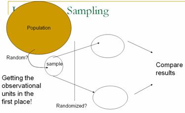
In this chapter, we transition from comparing two groups to focusing on how to sample the observational units from a population. While issues of generalizing from the sample to the population were touched in Chapter 1, in this chapter students formally learn about random sampling. We focus (but not exclusively) on categorical variables and introduce the binomial probability distribution in this chapter, along with more ideas and notation of significance testing. There is a new spate of terminology that you will want to ensure students have sufficient practice applying. In particular, we try hard to help students clearly distinguish between the processes of random sampling and randomization, as well as the goals and implications of each.

Section 3.1: Sampling from Populations I

Timing/Materials: Investigation 3.1.1 should take about one hour. We encourage you to have students use Minitab to select the random samples but they can also use the calculator or a random number table (if supplied). Investigation 3.1.2 can be discussed together quickly at the end of a class period, about 15 minutes. An applet is used in Investigation 3.1.3 and there are some Minitab questions in Investigation 3.1.4. These two investigations together probably take 60-75 minutes. You will probably want students to be able to use Minitab in Investigation 3.1.5 which can take 30-40 minutes. Exploration 3.1 is a Minitab exercise focusing on properties of different sampling methods (e.g., stratified sampling) which could be moved outside of class (about 30 minutes) or skipped. Investigation 3.1.2 and Exploration 3.1 can be regarded as optional if you are short on time.

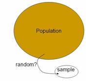
The goal of Investigation 3.1.1 is to convince students of the need for (statistical) random sampling rather than convenience sampling or human judgment. Some students want to quibble that part (a) only asks for “representative words” which they interpret as indicating representing language from the time or words conveying the meaning of the speech. This allows you to discuss that we mean “representative” as having the same characteristics of the population, regardless of which characteristics you will decide to focus on. Here we focus on length of words, expecting most students to oversample the longer words. Through constructing the dotplot of their initial sample means (again, we usually have students come to the front of the class to add their own observation), we also hope to provide students with a visual image of bias, with almost all of the student averages falling above the population average. We hope having students construct graphs of their sample data (in (d)) prior to the empirical sampling distribution (in (k)) will help them distinguish between these distributions. You will want to point out this distinction frequently (as well as insisting on proper horizontal labels of the variable for each graph – word length in (d) and average word length in (k)). We think it’s especially important and helpful to emphasize that the observational units in (d) are the words themselves, but the observational units in (k) are the students’ samples of words- this is a difficult but important conceptual leap for students to make. The sampling distribution of the sample proportions of long words in (k), due to the small sample size and granularity may not produce as a dramatic an illustration of bias, but will still help get students thinking about sampling distributions and sampling variability. This investigation also helps students practice with the new terminology and notation related to parameters and statistics. We often encourage students to remember that the population parameters are denoted by Greek letters, as in real applications they are unknown to the researchers (“It’s Greek to me!”). The goals of questions (r)-(w) are to show students that random sampling does not eliminate sampling variability but does eliminate bias by moving the center of the sampling distribution to the parameter of interest. By question (w) students should believe that a method using a small random sample is better than using larger nonrandom samples. Practice 3.1.1 uses a well-known historical context to drive this point home (You can also discuss Gallup’s ability to predict both the Digest results and the actual election results much more accurately with a smaller sample).

Investigation 3.1.2 is meant as a quick introduction to alternative sampling methods – systematic, multistage, and stratified. This investigation is optional, but you may even choose to talk students through these ideas but it’s useful for them to consider methods that are still statistically random but that may be more convenient to use in practice.

In the remainder of the text, we do not consider how to make inferences from any sampling techniques other than simple random sampling.

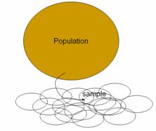
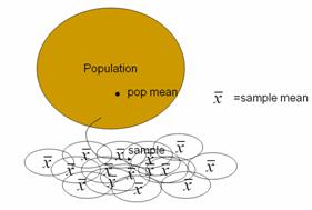
Investigation 3.1.3 introduces students to the second key advantage of using random sampling: not only does it eliminate bias, but it also allows us to quantify how far we expect sample results to fall from population values. This investigation continues the exploration of samples of words from the Gettysburg address using a java applet to take a much larger number of samples and to more easily change the sample size in exploring the sampling distribution of the sample mean. Students should also get the visual for a third distribution (beyond the sample and the empirical sampling distribution), the population. The questions step students through the sampling process in the applet very slowly to ensure that they understand what the output of the applet represents (e.g., what does each green square involve). The focus here is on the fundamental phenomenon of sampling variability, and on the effect of sample size on sampling variability; we are not leading students to the Central Limit Theorem quite yet. A common student difficulty is distinguishing between the sample size and the number of samples so you will want to discuss that frequently. 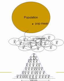Questions (m)-(p) attempt to help students to continue to think in terms of statistical significance by asking if certain sample results would be surprising; this reinforces the idea of an empirical p-value that arose in both Chapters 1 and 2. You may consider a simple PowerPoint illustration to help them focus on the overall process behind a sampling distribution (copy here), e.g.:

This exploration is continued in Investigation 3.1.4 but for sample proportions. Again the focus is on exploring sampling variability and sample size effects through the applet simulation. Beginning in (e) students are to see that the hypergeometric probability distribution describes the exact sampling distribution in this case. Students again use Minitab to construct the theoretical sampling distribution and expected value which they can compare to the applet simulation results. Students continue this comparison by calculating the exact probability of certain values compared to the proportion of samples simulated. Questions (o) and (p) ask students to again consider questions of what inferences can be drawn from such probability calculations. The subsequent practice problems address another common student misconception, that the size of the population always affects the behavior of the sampling distribution. In parts (a) and (c) of Practice 3.1.10, students consider using a sample of size 20 (and 2 nouns) instead of 100 words. We want students to see that with large populations, the characteristics of the sampling distribution do not depend on the population size (you will need to encourage them to ignore small deviations in the empirical values due to the finite number of samples).

In Investigation 3.1.5 students put what they have learned in the earlier investigations together by using the hypergeometric distribution to make a decision about an unknown population parameter based on the sample results and again consider the issue of statistical significance. In class discussion you will need to emphasize that this is the real application, making a decision based on one individual sample, but that their new knowledge of the pattern of many samples is what enables them to make such decisions (with some but not complete certainty). (Remind them that they usually do not have access to the population and that they usually only have one sample, but that the detour of the previous investigations was necessary to begin to understand the pattern of the sampling distribution.) In this investigation they are also introduced to other study design issues such as nonsampling errors. The graphs on p. 199 provide a visual comparison of the theoretical sampling distribution for different parameter values. You may want to circle the portion of the distribution to the right of the arrow, to help students see that the observed sample result is very unusual for the parameter value on the left (p = .5) but not for the one on the right (p = 2/3). The discussion tries to encourage students to talk in terms of plausible values of the parameter to avoid sloppy language like “p is probability is equal to 2/3.” You may want to remind them of what they learned about the definition of probability in Chapter 1 and how the parameter value is not what is changing in this process. The goal is to get students to thinking in terms of “plausible values of the parameter based on the sample results.”

As discussed above, Exploration 3.1 asks students to use Minitab to examine the sampling distribution resulting from different sampling methods. This could work well as a paired lab to be completed outside of class to further develop student familiarity and comfort with Minitab. One primary goal is for students to learn that stratification aims to reduce variability in sample statistics. Students should have completed the optional Investigation 3.1.2 before working on this exploration.

At this point in the course you could consider a data collection project where students are asked to take a sample from a larger population for a binary variable where they have a conjecture as to the population probability of success. Click here for an example assignment.

Section 3.2: Sampling from a Process

Timing/Materials: In this section we transition from sampling from a finite population to sampling from a process which motivates the introduction of the binomial probability distribution to replace the hypergeometric distribution as the mathematical model in this setting. Beginning in Investigation 3.2.2 we rely heavily on a java applet for simulating binomial observations and use both the applet and Minitab to compute binomial probabilities. This section should take 50-60 minutes, especially if you give them some time to practice Minitab on their own.

Investigation 3.2.1 presents a variation on a study that will be analyzed in more detail later. You may wish to replace the photographs at petowner.html (for Beth Chance, correct choice is in the middle) with your own. The goal here is to introduce a Bernoulli process and Bernoulli random variable; introduction of the binomial distribution waits until the next investigation. Investigation 3.2.2 presents a similar simulation but in a more artificial context which is then expanded to develop the binomial model. Rather than use the “pop quiz” with multiple choice answers but with no questions as we do, you could alternatively present students with a set of very difficult multiple choice questions for which you feel quite confident they would have to guess randomly at the answers. You can play up this example though, telling students to begin answering the questions immediately - they will be uncomfortable with the fact that you have not shown them any questions! You can warn them that question 4 is particularly tough J. The point is for the students to guess blindly (and independently) on all 5 questions. You can then show them an answer key (we randomly generate a different answer key each time) to have them (or their neighbor) determine the number of correct answers. You can also tease the students who have 0 correct answers that they must not have studied. You may want to lead the students through most of this investigation. Student misconceptions to look are for are confusing equally likely outcomes for the sample space with the outcomes of the random variable, not seeing the distinction between independence and constant probability of success, and incorrect application of the complement rule. The probability rules are covered very briefly. If you desire more probability coverage in this course, you may wish to expand on these rules.

In this investigation, we again encourage use of technology to help students calculate probabilities quickly and to give students a visual image of the binomial distribution. Questions (x) and (y) help students focus on the interpretation of the probability and how to use it to make decisions (is this a surprising result?), so this is a good time to slow down and make sure the students are comfortable. These questions also ask students to consider and develop intuition for the effects of sample size. They will again need to be reminded as in the hint in question (x) of the correct way to apply the complement rule. This comes up very often and causes confusion for many students. Question (aa) is also a difficult one for students but worth spending time on. The subsequent practice problems provide more practice in identifying the applicability of the binomial distribution and the behavior of the binomial distribution for different parameter values. Be specific with students as you use “parameter” to refer to both the numerical characteristic of the population and of the probability model.

Section 3.3: Exact Binomial Inference

Timing/Materials: This section will probably take about 3 hours, depending on how much exploring you want students to do vs. leading them through. Many students will struggle more than usual with all of the significance testing concepts and terminology introduced here, and they also need time to become comfortable with binomial calculations. Ideally students will have access to technology to carry out some of the binomial probability calculations (e.g., instructor demo, applet, or Minitab). Access to the applet is specifically assumed in Investigations 3.3.4 and 3.3.5 (for the accompanying visual images). Students are also introduced to the exact binomial p-value and confidence interval calculation in Minitab. Investigation 3.3.7 uses an applet to focus on the concept of type I and type II errors. Much of this investigation can be skipped though the definitions of type I and type II errors are assumed later.

Investigation 3.3.1 has students apply the binomial model to calculate p-values. We again have students work with questions reviewing the data collection process, some of which you may ask them to consider prior to coming to class. (There are many especially good measurement issues to discuss/debate with your students in these next few investigations.) We encourage you to be careful in helping students to understand what “success” and “failure” mean in this study because they are less straight-forward than in previous investigations: a “success” is a water quality measurement with a noncompliant dissolved oxygen level (less than 5.0 mg/l). Also be careful with the term “sample” here, because we use “sample” to refer to a series of water quality measurements rather than the conventional use of the term “water sample.” Because the actual study has a miniscule p-value, we begin in (f) by having students consider a subset of the data with less extreme results first, before examining the full dataset in (l). Once students feel comfortable with the steps of this inferential process (you may want to summarize the steps for them: start with conjecture, look at sample data, consider appropriate sampling distribution, calculate and interpret p-value as revealing how often the sample result would occur by chance alone if the conjecture were true), you can then add the terminology of the null and alternative hypotheses at the end of the investigation. You will want to get students into the habit of writing these hypothesis statements using both symbols and “in words.” You can draw the parallel that in Chs. 1 and 2, the null hypothesis was “no treatment effect.” In the terminology detour on p. 219, we start by consider the null as a set of values but then transition to always considering simple null hypothesis statements that specify equality to a single value of the parameter.

Students repeat this inferential process, and practice setting up null and alternative values in Investigations 3.3.2 (again considering issues of sample size) and 3.3.3 (a slightly more complicated, “nested” use of the binomial distribution). Again some students might find it disconcerting to define a “success” to be the negative result of a heart transplant patient who ended up dying. One point to make in question (k) of Investigation 3.3.2 is that the researchers tried to make a stronger case by analyzing data other than the original ten cases that provoked suspicion in the first place. Another point to make with this context is that the small binomial p-value enables us to (essentially) rule out random variation as the cause of the high observed mortality rate in this hospital, but we still have only observational data and so cannot conclude that the hospital is necessarily less competent than they should be. Perhaps a confounding variable is present; for example, the hospital might claim that they take on tougher cases than a typical hospital. But the binomial analysis does essentially prevent the hospital from claiming that their higher mortality rate is within the bounds of random variation. The graphs on p. 223 are a good precursor to considering when the binomial distribution can be approximated by a normal distribution (which comes up in Chapter 4). Also keep in mind that all of the alternative hypotheses up to this point have been one sided.

The transition to two-sided p-values is made in Investigations 3.3.4 and 3.3.5. You will want to help students understand when they will want to consider one-sided vs. two-sided alternatives. This is a trickier issue than when it’s presented in terms of a z-test, because here you don’t have the option of telling students to simply consider the test statistic value and its negative when conducting two-sided tests. In Investigation 3.3.4, the sampling distribution under the null hypothesis is perfectly symmetric (because that null hypothesis states that p = .5) but not in Investigation 3.3.5. In the former case, we consider the second tail to be the set of observations the same distance from the hypothesized value (or, equivalently, the expected value under the null hypothesis) as the observed result. But in the latter case, there are different schools of thought for calculating the two-sided p-value (as discussed on p. 231). The applet uses a different algorithm from Minitab. You may not want to spend long on this level of detail with your students, although some mathematically inclined students may find it interesting. Rather, we suggest that you focus on the larger idea of why two-sided tests are important and appropriate, and that students should be aware of why the two technologies (applet vs. Minitab) may lead to slightly different p-values. When using the binomial applet to calculate two-sided p-values, be aware that it may prompt you to change the inequality before it will do the calculation (to focus on tail extremes). Also be aware that the applet requires that you examine simulated results before it will calculate theoretical binomial probabilities.

Students enjoy the context of Investigation 3.3.5 and you can often get them to think about their own direction of preference, but we also try to draw the link to scientific studies in biomechanics. Note that we resist telling students about the sample results until after question (c); our point is that the hypotheses can (and should) be stated based on the research question before the observed data are even recorded. Be aware that the numerical values will differ slightly in (e) depending on the decimal expansion of 2/3 that is used. Question (e) of Investigation 3.3.5 anticipates the upcoming presentation of confidence intervals by asking students to test the plausibility of a second conjectured value of the parameter in the kissing study. We try hard to convince students that they should not “accept” the hypothesis that p = 2/3 in this case, but rather they should fail to reject that hypothesis and therefore consider 2/3 to be one (of many) plausible values of the parameter.

Investigation 3.3.6 then pushes this line of reasoning a step further by having students determine which hypothesized values of the parameter would not be rejected by a two-sided test. They thereby construct, through trial-and-error, an interval of plausible values for the parameter. We believe doing this “by hand” in questions (c) and (d), with the help of Minitab, will help students understand how to interpret a confidence interval. Many students consider this process to be fun, and we have found that some are not satisfied with two decimal places of accuracy and so try to determine the set of plausible values with more accuracy. A PowerPoint illustration of this process (but in terms of the population mean and the empirical rule) can be found here (view in slideshow mode). The applet can be used in a similar manner, but you have to watch the direction of the alternative in demonstrating this for students. The message to reiterate is that the confidence interval consists of those values of the parameter for which the observed sample result would not be considered surprising (considering the level of significance applied). Note that this is, of course, a different way to introduce confidence intervals than the conventional method of going a certain distance on either side of the observed sample result; we do present that approach to confidence intervals in Chapter 4 using the normal model.

Investigation 3.3.7 begins discussion on Types of Errors and power. You will want to make sure students are rather comfortable with the overall inferential process before using this investigation. Many students will struggle with the concepts but the investigation does include many small steps to help them through the process (meaning we really encourage you to allow the students to struggle with these ideas for a bit before adding your explanations/summary comments; you will want to make sure they understand the basic definitions before letting them loose). This investigation can also work well as an out of class, paired assignment. Our hope is that the use of simulation can once again help students to understand these tricky ideas. For example, in question (c), we want students to see that the two distributions have a good bit of overlap, indicating that it’s not very easy to distinguish a .333 hitter from a .250 hitter. But when the sample size is increased in (q), the distributions have much less overlap and so it’s easier to distinguish between the two parameter values, meaning that the power of the test increases with the larger sample size. The concept of Type I and Type II Errors will reoccur in Chapter 4.

Section 3.4: Sampling from a Population II

Timing/Materials: This section will take approximately one hour. Use of Minitab is assumed for parts of Investigations 3.4.1, 3.4.2, and 3.4.3.

In this section, students learn that the binomial distribution that they have just applied to random processes can also be applied to random sampling from a finite population if the population is large. In this way this section ties together the various sections of this chapter. Students consider the binomial approximation to the hypergeometric distribution and then use this model to approximate p-values. The goal of Investigation 3.4.1 is to help students examine circumstances in which the binomial model does and does not approximate the hypergeometric model well; they come to see how the probabilities are quite similar for large populations with small or moderate sample sizes. In particular, you will want to emphasize that with a population as large as all adult Americans (about 200 million people), the binomial model is very reasonable for sample sizes that pollsters use. Investigations 3.4.2 and 3.4.3 then provide practice in carrying out this approximation in real contexts. Investigation 3.4.3 introduces the sign test as another inferential application of the binomial distribution.

Summary

You will want to remind students that most of Ch. 3, calculating the p-values in particular, concerned binary variables, whether for a finite population or for a process/infinite population. Remind them what the appropriate numerical and graphical summaries are in this setting and how that differs from the analysis of quantitative data. This chapter has introduced students to a second probability model – binomial - to join the hypergeometric model from Chapter 1. If you will be concerned that students can properly verify the Bernoulli conditions, you will want to review those as well. Be ready for students to struggle with the new terminology and notation and proper interpretations of the p-value and confidence intervals. Encourage students that these ideas will be reinforced by the material in Ch. 4 and that the underlying concepts are essentially the same as they learned for comparing two groups in Chapters 1 and 2.

Another interesting out of class assignment here would be sending students to find a research report (e.g., http://www.firstamendmentcenter.org/PDF/SOFA.2003.pdf) and asking them to identify certain components of the study (e.g., population, sampling frame, sampling method, methods used to control for nonsampling bias and methods used to control for sampling bias), to verify the calculations presented, and to the comment on the conclusions drawn (including how these are translated to a headline).

Chapter 4

This chapter continues the theme of Chapter 3, the behavior of random samples from a population and how knowledge of that behavior allows us to make inferences about the population. Most of the chapter, beginning with Section 4.3, is devoted to models that apply when large samples are selected, namely the normal and t distributions. We begin with some background on probability models in general and the normal distribution in particular. Then we focus on the Central Limit Theorem for both categorical (binary) and quantitative data, leading students to discover the need for the t distribution when drawing inferences about the population mean. The last section, on bootstrapping, provides alternative inferential methods when the Central Limit Theorem does not apply (e.g., small sample, sample statistics other than sample proportions or means).

Section 4.1: Models of Quantitative Data

Timing/Materials: Heavy use of Minitab (including features new to version 14) is used in Investigation 4.1.1 and 4.1.2. You may want to assign some of the reading (e.g., p. 282-3) to outside of class. Probability plots (Investigation 4.1.2) may not be on your syllabus, but we ask students to use these plots often and so we do not recommend skipping them. This section can probably be covered in 60-75 minutes.

In this section we try to convey the notion of a model, in particular, probability models for quantitative variables. Investigation 4.1.1 introduces the idea that very disparate variables can follow a common (normal) model (with different parameter values). We do not spend a long time on nonnormal models (e.g., exponential, gamma) but feel students should get a flavor for nonsymmetric models as well and realize that the normal model does not apply to all variables. The subsequent practice problems lead students to overlay different model curves on data histograms. (Minitab 14 automatically scales the curve and thus we do not have them convert the histogram to the density scale first.).

In Investigation 4.1.2, probability plots are introduced as a way to help assess the fit of a probability model to data. There is some debate on the utility of probability plots, but we feel they provide a better guide than simple histograms for judging the fit of a model, especially for small data sets. Still, it can take students a while to become comfortable reading these graphs. We attempt to focus on interpreting these plots by looking for a linear pattern and do not ask students to learn the mechanics behind the construction of the graphs. We use questions (h)-(j) to help them gain some experience in judging the behavior of these graphs when the data are known to come from a normal distribution; many students are surprised at how much variation arises in samples, and therefore in probability plots, even when the population really follows a normal distribution. Some nice features in Minitab 14 make it easy to quickly change the model that is being fit to the data (both in overlaying the curve on the histogram and in the probability plot). If you are very short on time, Investigation 4.1.2 could be skipped but we will make use of probability plots in later chapters.

Section 4.2: Applying the (Normal) Probability Model

Timing/Materials: Minitab is used extensively in Investigations 4.2.1 and 4.2.2. Investigation 4.2.3 centers around a java applet which has the advantage of supplying the visual image of the normal model. You may wish to begin with Minitab until students are comfortable drawing their own sketches and thinking carefully about the scaling and the labeling of the horizontal axis. This section probably requires at least 90 minutes of class time (less if your students have seen normal probably calculations previously).

In Investigation 4.2.1, the transition is made to using the theoretical models to make probability statements. The last box on p. 290 will be an important one to emphasize. We immediately turn the normal probability calculation over to Minitab and do not use a normal probability table at all. (In fact, there is no normal probability table at all in the book as we do not feel that learning to use a table is necessary when students can use a software package or java applet (or even a graphing calculators) to perform the calculations quite efficiently. This also has implications for the testing environment.) We emphasize to students that it is important to continue to accompany these calculations with well-labeled sketches of probability curves and to distinguish between the theoretical probability and the observed proportion of observations in sample data. By the end of Investigation 4.2.1, we would like students to be comfortable applying a model to a situation where they don’t have actual observations. Such calculations are made in Practice Problems 4.2.1 and 4.2.2, including practice with elementary integration techniques and simple geometric methods for finding areas under probability “curves.” You could supplement this material with more on non-normal probability models, and you could make more use of calculus if you would like. In particular, you will find many of the exercises at the end of the chapter that explore more mathematical ideas, many involving use of calculus.

We continue to apply the normal probability model to real sample data in Investigation 4.2.2 and you will want to make sure students are becoming comfortable with the notation and Minitab. On p. 294, we discuss the complement rule for these continuous distributions and you will want to highlight this compared to the earlier adjustments for discrete distributions (once students “get” the discrete adjustment, they tend to over apply it). Beginning with question (i), this investigation also tries to motivate the correspondence between the probabilities calculated in terms of X from a N(m, s) distribution and in terms of Z from the Standard Normal distribution. This conversion may not seem meaningful to students at first (both for the ability to convert the measurements to the same scales and since we are not having them look the z-score up on a table) so you will want to remind them of the utility of reporting the z-value (presenting values on a common scale of standard deviations away from the mean, which enables us to “compare apples and oranges”). In using Minitab, most students will prefer using the menus but it may be worth highlighting some of the Session command short cuts as well. We have attempted to step students through the necessary normal probability calculations (including inverse probability calculations) but afterwards you will want to highlight the different types of problems and how they can recognize what is being asked for in a particular problem.

Exploration 4.2 provides more practice but using the java applet and could be completed by students outside of class. (If you use the latter option, be sure to clarify how much output you want them to turn in). You will want to make sure students are comfortable with the axis scales (note the applet reports both the x values and the z values) and in interpreting the probability that is reported. This investigation also introduces “area between” calculations and provides the justification of the empirical rule that students first saw in Chapter 2.

Section 4.3: Distributions of Sample Counts and Proportions

Timing/Materials: This section covers many important, and difficult for students, ideas related to the sampling distribution of a sample proportion. It introduces students to the normal approximation to the binomial distribution and to z-tests and z-intervals for a proportion. For Investigation 4.3.1, you will want to bring in Reese’s Pieces candies. You may be able to find the individual bags (“fun size”) or you may have to pour from a larger bag to each individual student. This takes some time in class but is always a student favorite. We often pour candies into Dixie cups prior to the start of class to help minimize the distribution time. We aim for at least 25 candies in each cup, and then ask students to select the first 25 “at random” (without regard to color). You can try to give these instructions before they have read too much about the problem context. Also in Investigation 4.3.1, they quickly turn to a java applet to take many more samples. Investigations 4.3.2 and 4.3.3 might actually be good ones to slowly step students through without the “distractions” of technology. Investigation 4.3.4 assumes students will use technology to calculate probabilities and you will want results from the earlier analysis of this study on hand. Similarly, technology is assumed for probability calculations in Investigation 4.3.5 including the 1 Proportion menu in Minitab. Exploration 4.3 involves the confidence interval simulation applet. Students can work through this together in pairs outside of class but you will want to insist on time in class for debriefing of their observations (and/or collection of written observations). You will want to carry out the “which prefer to hear first” survey in Investigation 4.3.6 to obtain the results for your students, possibly ahead of time. This investigation also requires quick use/demonstration of the confidence interval simulation applet. This section could take 3 hours of class time.

In Investigation 4.3.1, we first return to some very basic questions about sampling variability. Hopefully these questions will feel like review for the students but we think it is important to think carefully about these issues and to remind them of the terminology and of the idea of sampling variability. In (d), we often ask students to create a dotplot on the board, but you could alternatively type their results into Minitab and then project the graph to the class. Weaker students can become overwhelmed by the reliance on mathematical notation at this point and you will want to keep being explicit about what the symbols represent. In the investigation they are asked to think about the shape, center, and spread of the sampling distribution of sample proportions as well as using the applet to confirm the empirical rule. You should frequently remind students that the “observational units” are the samples here. They also think about how the sample size and the probability of success, p, affect the behavior of the sampling distribution. At this point students should not be surprised that a larger sample produces less variability in the resulting sample proportions.

Investigation 4.3.2 steps them through the derivations of the mean and standard deviation of the sampling distribution of a sample proportion including introduction to and practice for rules of expectation and variance. Mostly you will want to highlight how these expressions depend on n and p, and that the normal shape depends on both how large the sample size is and how extreme (close to 0 or 1) the success probability is. This (p. 310) is the first time students are introduced to the phrase “technical conditions” that will accompany all subsequent inferential procedures discussed in the course. You will probably have to give some discussion on why the normal approximation is useful since they already have used the binomial and hypergeometric “exact” distributions to make inferences. You might want to say that the normal distribution is another layer of approximation, just as the binomial approximates the hypergeometric in sampling from a large population. You might also highlight the importance of the normal model before the advent of modern computing. You will want to make sure everyone is comfortable with the calculations on p. 310, where all of the pieces are put together. Practice Problems 4.3.1 and 4.3.2 provide more practice doing these calculations and practice 4.3.3 is an optional exercise introducing students to continuity corrections.

Investigation 4.3.3 refers to the context of a statistical investigation and students must consider hypothesis statements and p-values, as they have before, but now using the normal model to perform the (approximate) calculations. You will want to emphasize that the reasoning process is the same. Some students will want to debate the “logic” of this context (for example, assuming that the proportion of women among athletes should be the same as the proportion of women among students, and the idea that the data constitute a sample from a process is not straight-forward here) and you will want to be clear about what this p-value does and does not imply and that there are many other issues involved in such a legal case (e.g., surveys of student interest and demonstrable efforts to increase the participation of women are also used in determining Title IX compliance). The idea of a test statistic is formally introduced on p. 313 (one advantage to using the normal distribution) and the discussion on p. 314 tries to remind students of the different methods for finding p-values with a single categorical variable that they have encountered so far. Students should be encouraged to highlight the summary of the structure of a test of significance p. 314-5 as one they will want to return to often from this point in the course forward. You might also want to show them how this structure applies to the earlier randomization tests from Chapter 1 and 2 as well.

Investigation 4.3.4 returns to an earlier study and re-analyzes the data with the normal approximation. You will want to have the reference for the earlier binomial calculation (from Investigation 3.3.5) handy. After question (h), this investigation continues on to calculate Type I and Type II Error probabilities through the normal distribution. Some students will find this treatment of power easier to follow than the earlier use of the binomial distribution, but you will want to make sure they are comfortable with the standard structure of tests of significance before continuing to these more subtle issues. We also suggest that you draw many pictures of normal curves and rejection regions to help students visualize these ideas, as with the sketches on p. 319.

Similarly, Investigation 4.3.5 shows how much more straight-forward it is to calculate a confidence interval using the normal model (though remind them that it still represents an interval of plausible values of the parameter). Students are introduced to the terms standard error and margin of error. This would be a good place to bring in some recent news reports (or have students find and bring in) to show them how these terms are used more and more in popular media. A subtle point you may want to emphasize with students is how “margin of error” and “confidence level” measure different types of “error.” You might want to emphasize the general structure of “estimate + margin of error” or “estimate + critical value × standard error” as described in the box on p. 324, for these forms arise again (e.g., with confidence intervals for a population mean).

Exploration 4.3 should help students to further understand the proper interpretation of confidence. This exploration can be completed outside of class, but you will probably want to emphasize to students whether you consider their ability to make a correct interpretation of confidence a priority. (We often tell them in advance it will be an exam question and warn them that it will be hard to “memorize” a definition due to the length of a correct interpretation and the insistence on context, so they should understand the process.) We hope the applet provides a visual image they will be able to use for future reference, for example by showing that the parameter value does not change but what does vary is the sample result and therefore the interval. Though we do want students to understand the duality between level of significance and confidence level, we encourage you to have them keep those as separate terms. One place you can trim time is how much you focus on sample size determination calculations, which are introduced in Practice Problem 4.3.9.

Investigation 4.3.6 provides students with a scenario where the normal approximation criteria (we expect) are not met and therefore an alternative method should be considered. We present the formula for the “Wilson Estimator” and then use the applet to have them explore the improved coverage properties of the “adjusted Wald intervals.” You may want to discuss with them some of the intuitive logic of why this would be a better method (but again focus on how the idea of confidence is a statement about the method, not individual intervals). In particular, in the applet, they should see how intervals that previously had length zero (because the sample proportion was 0 or 1), now produce meaningful intervals. Some statisticians argue that this “adjusted Wald” method should always be used instead of the original Wald method, but since Minitab does not yet have this option built in, and because the results are virtually identical for large sample sizes, we tend to have students consider it separately. We also like to emphasize to students how recently (since the year 2000 or so) this method has come into the mainstream to help highlight the dynamic and evolving nature of the discipline of statistics. We also like to emphasize out to students that they have the knowledge and skills at this point to investigate how well one statistical method performs compared to another.

All of these procedures (and technology instructions) are summarized on p. 334-5, another set of pages you will want to remind them to keep handy. Let students know if you will be requiring them to carry out these calculations in other ways.

Section 4.4: Distributions of Sample Means

Timing/Materials: Investigations 4.4.1 and 4.4.2 make heavy use of Minitab (version 14) with students creating more Minitab macros. Exploration 4.4 uses applets to visually reinforce some of the material in these first two investigations while also extending them. Use of Minitab is also assumed in Investigation 4.4.4, where you might consider having students collect their own shopping data for two local stores. A convenient method is to randomly assign each student a product (with size and brand details) and then ask them to obtain the price for their product at both stores. This appears to be less inconvenient for students than asking them to find several products, but you will still want to allow them several days to collect the data. These data can then be pooled across the students to construct the full data set. The sampling frame can be obtained if you can convince one local store to supply an inventory list or you can use a shopping receipt from your family or from a student (or a sample of students). This section will probably take at least 3 hours of class time.

This section parallels the earlier discussions in Section 4.3 but considers quantitative data and therefore focuses on distributions of sample means rather than proportions. It introduces students not only to the Central Limit Theorem for a sample mean but also to t-distributions, t-tests, and t-intervals, so it includes many important ideas. Students work through several technology explorations and you will want to help emphasize the “big picture” ideas. We believe that the lessons learned should be more lasting by having students make the discoveries themselves rather than being told (e.g., this distribution will be normal). In this section, students will be able to apply many of the simulation and probability tools and habits of mind learned earlier in the course. You will of course need to keep reminding students to carefully distinguish between the population, the sample, and the sampling distribution. You may also want to emphasize in Investigations 4.4.1 and 4.4.2 that these are somewhat artificial situations in that students are asked to treat the data at hand as populations and to take random samples from them; this is done for pedagogical purposes, but in real studies one only has access to the sample at hand.

Investigation 4.4.1 gives students two different populations, one close to normal and the other sharply skewed, and asks them to take random samples and study the distributions of the resulting sample means. Students who have become comfortable with Minitab macros will work steadily through the investigation, but those who have struggled with Minitab macros will move slowly and may need some help. When running the macro on p. 338, it is helpful to execute the macro once and create the dotplots of C2 and C3. If these windows are left open (and you have the automatic graph updating feature turned on), then when you run the macro more times, Minitab (version 14) should add observations to the windows and automatically update the displays. (This might be better as a demonstration.) Once students get a feel for how the samples are changing and how the sampling distribution is being built up, closing these windows on the fly will allow the macro to run much more quickly. Make sure that students realize the differences in results between the normal-looking and the skewed populations, which they are to summarize in (k). Once students have made the observations through p. 341, they are ready for the summary, the Central Limit Theorem. We try to emphasize that there’s nothing magical about the “n>30” criterion; rather we stress that the more non-normal the population, the larger the sample size needed for the normal approximation to be accurate. You will again need to decide if you want to present them with the formula s/, and have them verify that it matches the simulation results, and/or go through the derivation themselves. It is important to again give students plenty of practice in applying the CLT to solve problems (e.g., p. 342-3).

Investigation 4.4.2 then continues to have them explore coverage properties of confidence interval procedures and to motivate the need for t intervals to replace z intervals when the population standard deviation is unknown. We think that this is a discovery that is especially effective for students to make on their own; many students are surprised in (c) to see that the normal procedure does not produce close to 95% coverage here. Many students also find that the normal probability plots in (e) are very helpful, because it’s not easy to distinguish a t- from a z-distribution based on histograms/dotplots alone. After students make these observations, we always focus on t intervals (instead of z intervals) with sample means. Again, if you are short on time, you may want to streamline some of this discussion, but we also encourage you to use it as a vehicle to review earlier topics (e.g., confidence, critical values, technical conditions). In particular, you can remind them of the commonality of the general structure of the confidence interval, estimate + margin of error, or estimate + critical value × standard error

Exploration 4.4 is useful for providing students with visual images of the intervals while exploring coverage properties and widths (as in the previous investigation). This exploration also leads students to examine the robustness of t-intervals by considering different population shapes. The second applet asks them to explore how the t-interval procedure behaves for a uniform, a normal, and an exponential population. We want them to review the behavior of the sample and the sampling distribution (and be able to predict how each will behave) and hopefully by the end be able to explain why the sample size does not need to be as large with the (symmetric!) uniform distribution versus the exponential distribution to achieve the desired coverage.

Investigation 4.4.3 is intended as an opportunity for students to apply their knowledge and to make the natural leap to the one-sample t test-statistic. This is another good study to discuss some of the data collection issues. Also, in this case, the score of an individual game might be of more interest than the population mean and so we introduce the idea of a prediction interval and the formula for quantitative data. Be ready for students to struggle with the distinction between a confidence interval and a prediction interval. We do not show them a way to obtain this calculation from Minitab (because we don’t know one!). You should also remind students that the prediction interval method is much more sensitive to the normality condition. We do summarize the t procedures and technology tools on p. 359-360. You may want to give students the option of using either Minitab or the applet to perform such calculations. The applet has the advantage of automatically providing a sketch of the sampling distribution model which we feel you should continue to require as part of the details they include in their analyses. The applet also provides the 95% confidence interval more directly. In Minitab, you must make sure the alternative is set to “not equal” to obtain a two-sided confidence interval (we do not discuss one-sided intervals in the book) but Minitab also allows you to change the confidence level.

Investigation 4.4.4 introduces paired t procedures as an application of the above methods on the differences. This is a rich investigation that first asks students to conduct some data exploration and to consider outliers. There is an obvious outlier and when students look at the Data Window they find that the products were not actually identical. They can then remove such items (any where the size/brand combination does not match exactly) from the list before the analysis continues. You might want to emphasize that this type of exploration, cleaning, and data management is a large component of statistical analyses. While summarizing this investigation, you should emphasize the advantage of using a paired design in the first place.

Section 4.5: Bootstrapping

Timing/Materials: Heavy usage of Minitab is required in this section. Some of these ideas are very difficult for students, so you may want to lead them through this section more than most. If you do not have this enough time in your course, this section can be skipped, and later topics (except for Section 5.5, which could also be skipped) do not depend on students having seen these ideas.

Many advocate bootstrapping as a more modern, flexible procedure for statistical inference when the model based methods students have seen in this chapter do not apply. They also see bootstrapping as helping students understand the intuition of repeated sampling. Furthermore, instead of assuming a normally distributed sampling distribution, bootstrapping just relies on the “model” that the sample obtained reflects the population (and in fact assumes that the population is the sample repeated infinitely many times). In our brief experience in teaching bootstrapping (as an earlier topic in the course), we found it was difficult for students to get past the “sampling with replacement” philosophy and the theoretical details in a short amount of time. We subsequently moved the bootstrapping material to the end of Chapter 4 so that students would already by comfortable with the “traditional” procedures and the idea of sampling distribution. This will help them see how the bootstrapping approach differs while hopefully having enough background to understand the overall goals.

In Investigation 4.5.1, we begin by having students apply the theoretical results to the Gettysburg Address sampling to see that the normal/t distributions are not good models for smaller sample sizes. We provide more pictures/results than usual in this section but you can have students recreate the simulations themselves. Since the “sampling with replacement” approach feels mysterious to many students, we have them take a few samples to see that some words occur more than once and that we are just using an “infinite” population to sample from that has the same characteristics as the observed sample. Then we have them verify that the bootstrap distribution has the same shape and spread as the empirical sampling distribution of means. One way to approach bootstrapping is that it provides a way to estimate the standard error of a statistic (like the median or the trimmed mean) that do not have nice theoretical results (based on rules of variance). You can either stop here or you can continue on p. 369 to apply a “pivot method” to construct a bootstrap confidence interval. The notation becomes complicated and the results are not intuitive, but do help remind students of bigger issues such as the meaning of confidence and the effect of confidence level of the width of the interval. The bootstrap procedure is applied in Investigation 4.5.2. In Investigation 4.5.3 the behavior of the trimmed mean is explored, in a context where the mean is not a reasonable parameter to study due to the skewness and the truncated nature of the data. This “strange statistic” demonstrates a key advantage of bootstrapping (as well as the beauty of the CLT when it does apply). We found the 25% trimmed mean performs reasonably well. Carrying this calculation out in Minitab is a little strange but students should understand the commands in (d).

Examples

Note that this is the first chapter to include two worked-out examples. One deals with z-procedures for a proportion and the other with t-procedures for a mean. Earlier drafts did not include these examples, and students strongly requested that some examples be included, but we have since found that our students tend not to notice or study from the examples. You might encourage students to read them carefully, and especially to answer the questions themselves first before reading the model solutions provided.

Summary

The Chapter Summary includes a table on the different one-sample procedures learned for binary and quantitative data. With these students we like to use different notation (z* vs. z₀) to help them distinguish between critical values and test statistics, often a common source of confusion.

Exercises

Issues of probability distributions (as in Sections 4.1 and 4.2) are addressed in Exercises #1-20.  Issues of sampling distributions and inferences for a proportion are addressed in Exercises #21-46.  Issues of sampling distributions and inferences for a mean are addressed in Exercise #42 and #47-65.

Chapter 5

In this chapter, we focus on developing two-sample normal-based procedures, both for comparing two populations and for comparing two treatment groups. We again start with categorical data (Sections 5.1 and 5.2) before proceeding to quantitative data (Sections 5.3-5.5). We encourage you to again focus on the distinction between random sampling (Sections 5.1 and 5.3) and randomization (Sections 5.2 and 5.4), the corresponding impact on the scope of conclusions, and the place of inference in the entire statistical process (collecting data, analyzing data, including focusing on the appropriate numerical and categorical summaries, and then, if appropriate, inferential conclusions). Several points in this chapter allow students to combine many of the techniques they have learned throughout the course. Students should also be familiar with the pedagogical style of the course by now; for example, they should not be surprised that they are first asked about study design issues and about observational units and variables, and they then use simulation to come up with an empirical p-value, and they then examine the empirical sampling/randomization distribution and see if it can be approximated by a normal probability model. For students who have caught on to this approach, this chapter can proceed fairly quickly and demonstrate to them that they have “learned how to learn” about statistical methods.

Please note that the following timings are especially approximate as we have often done more jumping around in this chapter, often requiring students to work outside of class with these investigations. We do feel there is a tremendous amount of flexibility in how you use this chapter’s investigations in your own courses.

Section 5.1: Two Samples on a Categorical Response

Timing/materials: This chapter makes heavy use of Minitab (all but Investigation 5.1.2). Investigation 5.1.1 may take about 35 minutes as a student exploration but you can also lead students through the questions more quickly. Investigation 5.1.2, with help, may only take 15 minutes. On p. 417-8, students are stepped through using Minitab and an applet for these calculations. Investigation 5.1.3 can take about 50 minutes.

Investigation 5.1.1 helps students see that the binomial model they have been using with categorical data does not apply in analyzing the difference between two groups. The survey being conducted in two different years provides a nice context for emphasizing the independence of the samples. Notice that we still have students begin by considering questions of observational units and variable definitions. Students then use simulation in (j) to see that a normal model does provide a useful approximation for the difference in the sample proportions. As they have often in the course, students analyze the study data through an empirical p-value from their simulation.

Investigation 5.1.2 then steps students through the mathematical derivation of the mean and standard deviation of the sampling distribution of the difference in sample proportions, including a brief discussion of the Wilson adjustment. Since the content should look and feel familiar to the students by now, some of the details in this chapter could be presented to the students, rather than asking students to discover them through their own investigation, if you are quite short on time. You could focus on the technological tools for performing the calculations discussed on p. 417-418. The main ideas for students to understand are the setting of comparing two independent populations on a categorical response variable, why the normal model is useful, and how to interpret the computer output.

Investigation 5.1.3 steps students through the derivation of a confidence interval for an odds ratio. This investigation reinforces and combines many ideas from earlier in the course: case-control students, odds ratio as the most appropriate parameter in case-control studies, simulation of an empirical sampling distribution of the sample statistic, transformations to normalize a distribution, and construction of a normal-based confidence interval using the form: estimate ± (critical value × standard error of statistic). We again start students by considering study design issues before even revealing the study results. The journal article can be found at http://bmj.com/cgi/content/full/324/7346/1125. The researchers in this study conducted the interviews with case drivers in the hospital room or by telephone; they say only that proxies were used for drivers who had died. They defined a full night’s sleep to be at least seven hours, mostly between 11pm and 7am. They also used several other measures of sleep, specifically the Stanford and Epworth sleepiness scales, in case you would like students to look up the journal article and analyze some other variables. Note that the sample size for the “case” drivers given on the bottom of p. 421 is smaller than that reported on p. 420, reflecting the nonrespondents. Also note the typo on p. 422, the sample odds ratio is 1.59, not 1.48. In the simulation conducted in (i), each row will represent a new two-way table. Remember that the simulation assumes a value for the common population proportion and that also motivates an advantage of the more general normal based model which applies for any value of p. Many students are surprised in (i) that this time, unlike so many earlier investigations, the sampling distribution of this statistics (odds ratio) is not well approximated by a normal distribution, and we hope that students will think of applying a transformation to make the distribution more normal. We made the decision to simply tell students the formula for the standard error but you may want to go through the derivation with more mathematically inclined students. In (m), we ask for a 90% confidence interval, but you could consider a 95% confidence interval as well [(1.06, 2.39)]. You may need to remind students to “back-transform” with exponentiation in order to produce a confidence interval for the odds ratio rather than the log odds ratio. Another point to remind them of is that it’s relevant to check whether the interval includes the value one, rather than the value zero as with a difference in proportions.

Section 5.2: Randomized Experiments Revisted

Timing/materials: Investigation 5.2.1 requires a Minitab macro (and letrozole.mtw) but may only take about 30 minutes.

Section 5.2 transitions from independent random samples to randomized experiments, but you might remind students that this scenario was already discussed in Ch. 1. Students should recall that the hypergeometric distribution for Fisher’s exact test often looked fairly symmetric and normal. Here, we focus on using the normal model as a large sample approximation to Fisher’s exact test, complete with null and alternative hypothesis statements about the treatment effect, d. The normal-based model also has the advantage of providing a direct method for determining a confidence interval for the size of the treatment effect.

In Investigation 5.2.1, students use a macro to obtain an empirical sampling distribution for both the difference in group proportions and the sample odds ratio. You may wish to provide them with an existing file to execute instead of asking them to take the time to type all the commands in. Students are also reminded that the normal-based method also provides a test statistic as an additional measure of the extremeness of the sample result. Otherwise, you can caution them that there are not a lot of current advantages to using the large sample method but that previously (before modern computers) Fisher’s exact test was computationally intensive with large sample sizes. The details for using Minitab or an applet to carry out the z-procedures are given on p. 431. Once again, you might want to emphasize that the randomization in the experimental design allows for drawing causal conclusions when the difference in the groups turns out to be statistically significant.

Section 5.3: Comparing Two Samples on a Quantitative Response

Timing/materials: Investigation 5.3.1 also requires a Minitab macro that students create to use with NBASalaries0203.mtw, and Investigation 5.3.2 requires features that are new to Version 14 of Minitab. These two activities together should take 50-60 minutes. Investigation 5.3.3 (shopping99.mtw) should only take about 15 minutes.

Section 5.3 transitions to comparing two groups generated from independent random samples on a quantitative response variable. It might be useful to highlight the different contexts they will examine in this section (NBA salaries by conference, body temperatures of men vs. women, life expectancy of right and left handers) to help them understand the settings in which these techniques will apply. In Investigation 5.3.1, students again first examine simulation results and then consider the theoretical derivations of the mean and expected value. This is another situation, as with the Scottish militiamen and mothers’ ages, where we give students access to an entire population and ask them to repeatedly take random samples from it. You might want to remind students that this is a pedagogical device for studying sampling distributions; in real life we would only have access to one sample, and if we did have access to the whole population there would be no need to conduct inference. By the end of this investigation, we remind them of the utility of the t distribution with quantitative data. Again you may choose to present these results to students more directly if you are short on time. It will be important that they at least read through the “Probability Detour” on p. 436-7. You will probably also want to remind them of how Minitab handles stacked and unstacked data. We encourage you not to short change the discussion of the numerical and graphical summaries and what they imply to contrast what the inferential tools tell them.

Investigation 5.3.2 presents an interesting application of the two-sample t-statistic, assuming use of Minitab 14, where only the sample means and sample standard deviations need to be specified (as opposed to the raw data). If Minitab 14 is not available, you may consider having different students carry out the calculations for the different scenarios by hand. The point is to make sure the students have time to describe the effects of the sample standard deviations and the relative sample sizes in the two groups on the test statistic and p-value. You can also engage in a class discussion about which scenarios seem “plausible.” Most students will agree that sample standard deviations of 50 do not make much sense with means of 66 and 75, because even though the distribution of lifetimes may not be symmetric, we might expect the minimum to be further than just one standard deviation from the mean. Students will also debate the reasonableness of the different percentages of left-handers. The point we hope to make is even if we don’t know these values exactly (they truly were not reported in this study), we can still make some tentative conclusions about the significance of the result. Of course, you will still want to emphasize in class discussions that a statistically significant result is not sufficient, due to the observational nature of the study, to imply a cause and effect result. Questions (j) and (k) also reinforce this point. The context of this investigation is interesting to students, though be wary of sensitivity issues. Students will often have opinions (especially left-handed students) related to this study. You can also bring in some of the “history” of this type of research and some of the doubts of its validity (see p. 441). Practice Problem 5.3.3 provides practice with a similar context with a reminder of statistical vs. practice significance (“Should students pay money to be able to increase their scores by 65 points?”) that may be worthwhile to reinforce in class.

Investigation 5.3.3 provides another application of the two-sample t test by again analyzing the comparison shopping data, this time focusing on the price differences. The crucial point, which arises in (c) and (d), is that the earlier methods of Chapter 5 do not apply because of the paired (and therefore non-independent) nature of the data collection. This context has been used several times and you may want to compare the results of the different analyses (e.g., sign test vs. two-sample t test) as in (j). It’s also important to emphasize the difference between a statistically significant difference and a practically significant difference as in (i) where they are asked to comment on whether an average price difference per item of $.03 to $.29 is worthwhile. You can ask them to consider how much farther away the cheaper store would need to be for such a difference to no longer be worthwhile. The Practice Problems also provide a few additional applications of the t-procedures for comparing paired quantitative data, but you may want to add a few more/be ready to provide help on HW problems. Be sure not to miss the t-procedure summary on p. 452-3.

Section 5.4: Randomized Experiments Revisited

Timing/materials: Investigation 5.4.1 only requires analysis of the data in SleepDeprivation.mtw from Chapter 2. Exploration 5.4 also uses Minitab.

Section 5.4 mirrors Section 5.2 in that it demonstrates that the t-distribution provides a reasonable approximation to the randomization distribution. In Investigation 5.4.1 students are presented with the relevant output to see this, returning to the sleep deprivation study for which they approximated a randomization test near the end of Chapter 2. If you have more time, you may want students to help create this output for themselves. You may remind students that near the end of Chapter 2, they were actually shown the picture of a t-distribution (p. 148) to foreshadow what they are now learning in this section. We initially show the parallel with the pooled t-test but in general do not recommend pooling even with experimental data as the benefits do not appear to outweigh the risks. This is also a good point to remind students that in writing their final conclusions they should focus on whether the difference is statistically significant, the population(s) the results can be generalized to and whether a cause-and-effect conclusion can be drawn.

Exploration 5.4 can be considered optional. The exploration asks students to examine various approximations for the (unknown) exact degrees of freedom in non-pooled, two-sample t-procedures. This exploration may appeal to more mathematically inclined students who want to examine the relative merits of different approximations that are recommended.

Section 5.5: Other Statistics

Timing/materials: Investigation 5.5.1 also uses macros and will take about 20 minutes.

Section 5.5 can also be considered optional as it returns to the issue of bootstrapping, this time in the two sample case. The case is made that this approach may be advantageous when something other than the difference in sample/group means is of interest. In Investigation 5.5.1 the difference in group medians is considered for “truncated” data (not all response times will be completed by the time of the end of the study), where it’s impossible to calculate group means directly. Students create an empirical bootstrap distribution and see that it is not normal and then proceed to consider a bootstrap percentile interval. The simulations again emphasize whether we want to model the data as coming from two independent samples or from random assignment. Both of these approaches are hypothetical for this particular observational study, but students can see that the conclusions about statistical significance would be similar. We do not go into extensive data on the bootstrapping procedures, e.g., bias-corrected methods) but if this is a year long course for your students this could be a good place to expand the discussion.

Examples

There are two examples here, one highlighting a comparison of proportions and one highlighting a comparison of means.

Summary

At the end of this chapter it will be important to highlight how the appropriate procedure follows from the study design and the type and number of variables involved. We encourage you to give students a mixture of problems where deciding on t-test vs. z-test is not always transparent. Similarly for one-sample (matched pairs) and two-sample procedures. (We especially like exercise 15 for focusing on this issue as well as reminding them of important non-computational issues such as question wording in surveys.) Students will also need to be reminded on when and why they might want to consider Fisher’s exact test. Since this chapter focused mostly on methods, it will also be important to remind them not to ignore some of the larger issues such as interpreting statistical significance, type I and type II errors, association vs. causation, meaning of confidence, scope of conclusions, etc.

Exercises

Issues of comparing proportions (as in Sections 5.1 and 5.2) are addressed in Exercises #1-22 and #35.  Issues of comparing means (as in Sections 5.3 and 5.4) are addressed in Exercises #22-43.  Exercises #22 and #35 concern issues of both types of analyses.

Chapter 6

This chapter again extends the lessons students have learned in earlier chapters to additional methods involving more than one variable. The material focuses on the new methods (e.g., chi-square tests, ANOVA, and regression) and follows the same progression as earlier topics: starting with including appropriate numerical and graphical summaries, proceeding to use simulations to construct empirical sampling/randomization distributions, and then considering probability models for drawing inferences. The material is fairly flexible if you want to pick and choose topics. Fuller treatments of these methods would require a second course.

Section 6.1: Two Categorical Variables

Timing/materials: Minitab and a macro (SpockSim.mtb) are used in Investigation 6.1.1. Minitab is used to carry out a chi-square analysis in Investigations 6.1.2 and 6.1.3. These three investigations may take about 90-100 minutes, with Investigation 6.1.1 taking about 50-60 minutes. Exploration 6.1 revolves around a Minitab macro (twoway.mtb which uses worksheet refraction.mtw).

The focus of this section is on studies involving two categorical variables and in particular highlights different versions of the chi-square test for tables larger than 2 × 2. In Investigation 6.1.1 you may want to spend a bit of time on the background process of the jury selection before students analyze the data. We also encourage you again to stop and discuss the numerical and graphical summaries that apply to these sample data (question (a)) before proceeding to inferential statements, as well as reconsidering the constant theme – could differences this large have plausibly occurred by chance alone? After question (h), you will also want to explain the logic behind the chi-square statistic – every cell gives a positive contribution to the sum but it is also scaled in a way by the size of the cell’s expected cell count. If students follow the formula, question (j) should be straight forward to them. After thinking about the behavior based on the formula, we then use simulation as a way of judging what values of the statistic should be considered large enough to be unusual and also to see what probability distribution might approximate the sampling distribution of the test statistic. Because we are simulating the drawing of independent random samples from several populations, we use the binomial distribution, as opposed to treating both margins as fixed like we did in Chapter 1. We have given students the macro to run (SpockSim.mtb) in question (k), but you may want to spend time making sure they understand the workings of the Minitab commands involved and the resulting output. The simulation results are also used to help students see that the normal distribution does not provide a reasonable model of the empirical sampling distribution of this test statistic. We do not derive the chi-square distribution but do use probability plots to show that the Gamma distribution, of which the chi-square distribution is a special case, is appropriate (questions (n) and (o)). Again, we want them to realize that the probability model applies no matter the true value of the common population proportion p. We also encourage them to follow-up a significant chi-square statistic by seeing which cells of the table contribute the most to the chi-square sum as a way of further defining the source(s) of discrepancy (questions (q) and (r)). There is a summary of this procedure on p. 490 along with Minitab instructions. The section of Type I Errors on p. 491 is used to further motivate the use of this “multi-sided” procedure for checking the equality of all population proportions simultaneously.

Investigation 6.1.2 provides an application of the chi-square procedure using Minitab but in the case of a cross-classified study first examined in Chapter 1. You might want to start by asking them what the segmented bar graph would have looked like if there was no association between the two variables. The details of the chi-square procedure are summarized, with Minitab instructions, on p. 494-5 and you may wish to give students additional practice, in addition to the practice problems, especially in distinguishing these different situations (e.g., reminding them of the different data collection scenarios, the segmented bar graphs, the form of the hypotheses – comparing more than 2 population proportions, comparing population distributions on a categorical variable, association between categorical variables).

Investigation 6.1.3 focuses on the correspondence between the chi-square procedure for a 2 × 2 table and the two-sample z-test with a two-sided alternative.

Exploration 6.1 may be considered optional but is meant to illustrate that the chi-square distribution is appropriate for modeling the randomization distribution (corresponding to Investigation 6.1.2) as well as the sampling distribution (as in Investigation 6.1.1). Students are given a macro to run but are asked to explain the individual commands.

Section 6.2: Comparing Several Population Means

Timing/materials: Minitab is used for descriptive statistics (HandicapEmployment.mtw) and a Minitab macro (RandomHandicap.mtb) is used in Investigation 6.2.1. Minitab is used again at the end of the investigation to carry out the ANOVA. Minitab can be used briefly in Investigation 6.2.2 to calculate a p-value from the F distribution. The ANOVA simulation applet is also used heavily. This section should take about 65 minutes.

The focus on this section is on comparing 2 or more population means (or treatment means). You may want to cast this as the association between one categorical and one quantitative variable to parallel the previous section (though some suggest only applying this description with cross-classified studies). Again, we do not spend a large amount of time developing the details, seeing these analyses as straight forward implementations of previous tools with slight changes in the details of the calculation of a test statistic. We hope that students are well-prepared at this point to understand the reasoning behind the big idea of comparing within-group to between-group variation, but you might want to spend some extra time on this principle. You will also want to focus on emphasizing all the steps of a statistical analysis (examination of study design, numerical and graphical summaries, and statistical inference including defining the parameters of interest, stating the hypotheses, commenting on the technical conditions, calculation of test statistic and p-value, making a decision about the null hypothesis, and then finally stating an overall conclusion that touches on each of the issues).

Investigation 6.2.1 steps students through the calculations and comparison of within group and between group variability and uses a macro to examine the empirical sampling distribution of the test statistic. Question (o) is a key one for assessing whether students understand the basic principle. More details are supplied in the terminology detour on p. 506 and general Minitab instructions for carrying out an ANOVA analysis are given on p. 507.

In Investigation 6.2.2, students initially practice calculating the F-statistic by hand. Then a java applet is used to explore the effects of sample size, size of the difference in population means, and the common population variance on the ANOVA table and p-value. We have tried to use values that allow sufficient sensitivity in the applet to see some useful relationships. It is interesting for students to see the variability in the F-statistic and p-value from sample to sample both when the null hypothesis is true and when it is false. An interesting extension would be to collect the p-values from different random samples and examine a graph of their distribution, having students conjecture on its shape first.

Practice Problem 6.2.1 is worth emphasizing; its goal is to help students understand why we need a new procedure (ANOVA) here in the first place, as opposed to simply conducting a bunch of two-sample t-tests on all pairs of groups. Practice Problem 6.2.2 demonstrates the correspondence of ANOVA to a two-sided two-sample t-test, when only two groups are being compared, and is worth highlighting. An interesting in-class experiment to consider in the section on ANOVA is the melting time of different types of chips (e.g., milk chocolate vs. peanut butter vs. semi-sweet, similar to the study described in Exercise 46 in Chapter 3), especially considering each person as a blocking factor (and are willing to discuss “two-way” ANVOA). You might also consider at least demonstrating multiple comparison procedures to your students.

Exercise 59 is a particularly interesting follow-up question, re-analyzing the Spock trial data using ANOVA instead of Chi-square, and considering how the two analyses differ in the information provided.

Section 6.3: Relationships Between Quantitative Variables

Timing/materials: Minitab is used for basic univariate and bivariate graphs and numerical summaries in Investigation 6.3.1 (housing.mtw). Minitab is used to calculate correlation coefficients in Investigation 6.3.2 (golfers.mtw). These two investigations may take about 45 minutes. Exploration 6.3.1 revolves around the Guess the Correlation applet and will take 10-15 minutes. Investigation 6.3.3 uses the Least Squares Regression applet and at the end shows them how to determine a regression equation in Minitab (HeightFoot.mtw) and can take upwards of 60 minutes. Investigation 6.3.4 also involves Minitab (movies03.mtw) and may take 30 minutes. Exploration 6.3.2 revolves around the Least Squares Regression applet and Exploration 6.3.3 uses Minitab (BritishOpen00.mtw).

This section presents tools for numerical and graphical summaries in the setting of two quantitative variables. Here we are generally less concerned about the type of study used. The next section will focus on inference for regression.

Investigation 6.3.1 focuses on using Minitab to create scatterplots and then introducing appropriate terminology for describing them. Investigation 6.3.2 uses data from the same source (PGA golfers) to explore varying strengths of linear relationships and then introduces the correlation coefficient as a measure of that strength. One thing to be sure that students understand is that low scores are better than high scores in golf; similarly a smaller value for average number of putts per hole is better than a larger value, but some other variables (like driving distance) have the property that higher numbers are generally considered better. Discussion in this investigation includes how the points line up in different quadrants as a way of visualizing the strength of the linear relationship. Question (i) is a particularly good one to give students a few minutes to work through on their own in collaborative groups. Students should also be able to describe properties of the formula for r (when positive, negative, maximum and minimum values, etc.); in fact, our hope in (k)-(n) is that students can quickly tell you these properties rather than you telling them. Students apply this reasoning to order several scatterplots in terms of strength and then use Minitab to verify their ordering. If you want students to have more practice in estimating the size of the correlation coefficient from a scatterplot, Exploration 6.3.1 generates random scatterplots, allows students to specify a guess for r and then shows them the actual value. The applet keeps track of their guesses over time (to see if they improve) as well as the guesses vs. actual and errors vs. actual to see which values of r were easier to identify (e.g., closer to -1 and 1). Questions (g)-(i) also get students to think a bit about the meaning of r. Students often believe they are poor guessers and that the correlation between their guesses and the actual values of r will be small. They are often surprised at how high this correlation is, but should realize that this will happen as long as they can distinguish positive and negative correlations and that they may find a high correlation if they guess wrongly in a consistent manner. Practice Problem 6.3.1 is a very quick test of students’ understanding; question (b) in particular confuses many students. A Practice Problem like 6.3.2 is important for reminding them that r measures the amount of the linear association.

Investigation 6.3.3 steps students through a development of least squares regression. Starting after (g), they use a java applet with a moveable line feature to explore “fitting the best line” and realize that finding THE best line is nontrivial and even ambiguous, as there are many reasonable ways to measure “fit.” We emphasize the idea of a residual, the vertical distance between a point and the line, as the foundation for measuring fit, since prediction is a chief use of regression. In question (k) we briefly ask students to consider the sum of absolute residuals as a criterion, and then we justify using SSE as a measure of the prediction errors. Parallels can be drawn to Exploration 2.1 (p. 133). In questions (k)-(m) many students enjoy the competitive aspect of trying to come up with better and better lines according to the two criteria. Students can then use calculus to derive the least squares estimators directly in (p) and (q). Questions (s) and (t) develop the interpretation of the slope coefficient and question (u) focuses on the intercept. Question (v) warns them about making extrapolations from the data. The applet is then used in questions (w) and (x) to motive the interpretation of r². Spacing left in the book for written responses to these questions is probably smaller than it should be. Once the by-hand derivation of the least squares estimates are discussed, instructions are given for obtaining them in Minitab. Investigation 6.3.4 provides practice in determining and interpreting regression coefficients with the additional aspect, which students often find interesting, of comparing the relationship across different types of movies.

Exploration 6.3.2 uses an applet to help students visualize the influence of data values, particularly those with large x-values, on the regression line. Exploration 6.3.3 introduces students to the “regression effect.” There is a nice history to this feature of regression and it also provides additional cautions to students about drawing too strong of conclusions from their observations (e.g., “regression to the mean”). We often supplement this discussion with excerpts from the January 21, 2001 Sports Illustrated article on the cover jinx.

“It was a hoot to work on the piece. On the one hand, we listened as sober statisticians went over the basics of ‘regression to the mean,’ which would explain why a hitter who gets hot enough to make the cover goes into a slump shortly thereafter.”

Section 6.4: Inference for Regression

Timing/materials: Minitab is used in Investigation 6.4.1 (hypoHt.mtw) and Investigation 6.4.2 (housing.mtw). Together, these investigations can take less than 30 minutes. Investigation 6.4.3 revolves around the Simulating Regression Lines applet and takes 35-45 minutes. Investigation 6.4.4 really just requires a calculator (Minitab output is supplied) and takes about 20 minutes.

This section finishes the discussion of regression by developing tools to make inferential statements about a population regression slope. Investigation 6.4.1 begins by having students consider the “ideal” setting for such inferences – normal populations with equal variance that differ only in their means that follow a linear pattern with the explanatory variable. We especially advocate the LINE mnemonic. Residual plots are introduced as a method for checking the appropriateness of this basic regression model. Investigation 6.4.2 then applies this model to some student collected data. The linearity condition does not appear met with these data and we have them perform a log-log transformation. If you think this transition will be too challenging for your students, you may want to provide more linear examples first. Details for why the log-log transformation is appropriate and for interpreting the resulting regression coefficients in terms of the original variables are left for a second course. In this section we are more concerned that students can check the conditions and realize that additional steps can be taken when they are not met and we try not to get too bogged down at this time in interpreting the transformation.

Investigation 6.4.3 follows the strategy that we have used throughout the course: taking repeated random samples from a finite population in order to examine the sampling distribution of the relevant sample statistic. We ask students to use a java applet to select random samples from a hypothetical population matching the house price setting that follows the basic regression model, but where the population has been chosen so that the correlation (and therefore the slope) between log(price) and log(size) is zero. The goal of the applet is for students to visualize sampling variability with regression slopes (and lines) as well as the empirical sampling distribution of the sample slopes. This process should feel very familiar to students at this point, although you should be aware that it feels different to some students because they are watching sample regression lines change rather than seeing simpler statistics such as sample proportions or sample means change. Students also explore the effects of sample size, variability in the explanatory variable and variability about the regression line on this sampling distribution. This motivates the formula for the standard error of the sample slopes given on p. 550. It is interesting to help students realize that when choosing the x values, as in an experiment, more variability in the explanatory variable is preferred, a sometimes counter-intuitive result for them. Students should also note the symmetry of the sampling distribution of sample slope coefficients and believe that a t-distribution will provide a reasonable model for the standardized slopes using an estimate for the standard deviation about the regression line. Students calculate the corresponding t-statistic for the house price data by hand.

Investigation 6.4.4 then further focuses on the corresponding Minitab output. Questions (f)-(l) also deal with confidence intervals for slope and confidence intervals and prediction intervals (and the distinction between them, for which you can draw the connection to univariate prediction intervals from Chapter 4) for individual values. Minitab provides for nice visuals for these latter intervals. The bow-tie shape they saw in the applet is also a nice visual here for justifying the “curvature” seen especially in prediction intervals.

Examples

This chapter includes four worked-out examples. Each of the first three deals with one of the three main methods covered in this chapter: chi-square tests, ANOVA, and regression. The fourth example analyzes data from a diet comparison study, where we ask several questions and expect students to first identify which method applies to a given question. Again we encourage students to answer the questions and analyze the data themselves before reading the model solutions.

Summary

At the end of this chapter, students will most need guidance on when to use each of the different methods. The table on p. 571 may be useful but students will also need practice identifying the proper procedure merely from a description of the study design and variables. We also like to remind students to be very conscious of the technical conditions underlying each procedure and that they must be checked and commented on in any analysis.

Exercises

Section 6.1 issues are addressed in Exercises #1-16 and #61.  Section 6.2 issues are addressed in Exercises #17-30 and #59 and #62.  Section 6.3 and 6.4 issues are addressed in Exercises #31-60 and #63.  Exercises #60-62 ask students to perform all three types of analyses (chi-square, ANOVA, regression) on the same set of data, and Exercise #59 asks for an ANOVA analysis of data previously analyzed with a chi-square procedure. NOTE: The data file for “ComparingDietsFull.mtw” on the CD does not contain all of the necessary variables to complete Exercise 29. A newer version of the data file can be download from the ISCAM Data Files page.