Unit II - In-Class Activities

7-1: Cars Fuel Efficiency ( cont. )

(a)

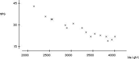
(b) Heavier cars tended to get worse fuel efficiency.

(c) negatively

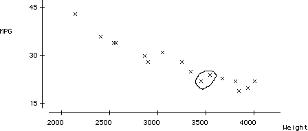
(d) yes; there are many such pairs.

7-2: Guess the Association

(a) Students who did well on the first test tended to do well on the second, and those who did poorly on the first tended to do poorly on the second.

(b)

(c) (Asks for interpretation)

7-3: Marriage Ages ( cont. )

(a) yes; positive; fairly strong

(b) 2

(c) 16

(d) 6

(e) One can discover that for most of these couples, the husband is older than the wife.

7-4: Space Shuttle O-Ring Failures

(a)

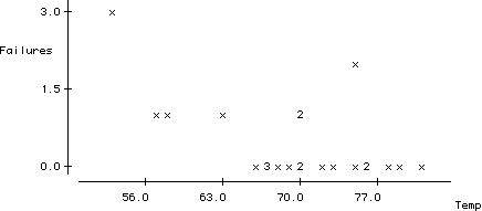
The scatterplot reveals a weak-to-moderate negative association between temperature and O-ring failures.

(b) The likelihood of O-ring failure appears to be greater at such a low temperature.

(c)

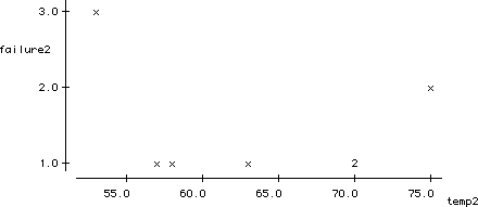
The association is much weaker in this case.

(d) (Asks for interpretation)
 

7-5: Fast Food Sandwiches

(a)

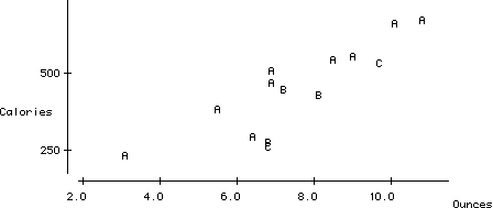
A- roast beef
B - chicken
C - turkey

(b) There is a reasonably strong, positive association between a sandwich's serving size and its calories.

(c) Roast beef sandwiches tend to have more calories per serving size than do chicken and turkey sandwiches.

8-1: Properties of Correlation

(a)-(b)

(c) largest: 1; smallest: -1

(d) The data would have to fall exactly on a straight line.

(e) The sign of the correlation (positive or negative) matches the direction of the association.

(f) The stronger the association, the closer the correlation comes to ±1. The weaker the association, the closer the association comes to 0.

(g) The data reveal a distinct curvilinear relationship.

(h) 0

(i) Yes, except for the person who scored very high on the first exam and very low on the second.

(j) Yes, except for the person who scored very low on both exams.

(k) H: 0.037; I: 0.705

(l) H: 1.000; I: 0.130; These correlations have changed substantially.

(m) No, because it can be strongly affected by outliers.

(n) There are two distinct clusters, one with students doing poorly on both exams and another with students doing well on both exams.

(o) .954

8-2: Televisions and Life Expectancy

(a) fewest: United States, 1.3; most: Haiti, 234

(b)

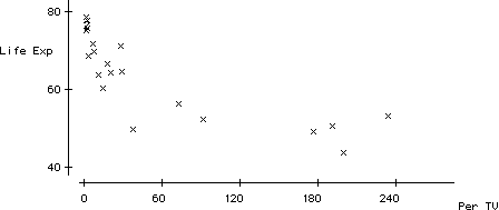
(c) -.804

(d) (Asks for interpretation)

(e) no

(f) (Asks for interpretation)

8-3: Cars' Fuel Efficiency ( cont. )

(a)

(b) -.96

(c) The cars with negative weight z-scores tend to have positive MPG z-scores, and vice versa.

8-4: Guess the Correlation

(a) - (g) The answers vary from student to student.

(e) If guesses are on the vertical axis, then points above the line indicate overestimates.

(h) one

(i) one

(j) no, see (h) and (i)

9-1: Air Fares ( cont. )

(a) - (e) The answers vary from student to student.

9-2: Air Fares ( cont. )

(a)

(b) b = 0.117; a = 83.3

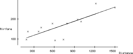
(c) airfare = 83.3 + .117 distance

(d) Should match (may differ slightly due to rounding)

(e)118.50

(f) 259.30

(g)-(h)

(i) (Asks for prediction)

(j) 188.90

(k) 416.80

(l)

(m) yes; 0.117; this number is the slope coefficient of the least squares line.

(n) 11.70

(o) 150.88

(p) 27.12

(q)

(r) St. Louis; distance: 737 airfare: 98; residual: 71.77; overestimate

(s) greater

(t) below

(u) mean: 0; standard deviation: 36.1

(v) 0.368

(w) 0.632

(x) The sum equals one.

(y) .632

9-3: Students' Measurements ( cont. )

(a) - (e) These answers depend on class results.

(f) no

10-1: Gestation and Longevity

(a)

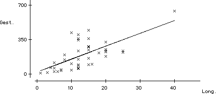
Gestation = 21.7 + 13.1 Longevity

(b) For every additional year of longevity, one expects the animal's gestation period to increase by 13.1 days.

(c) .44

(d)

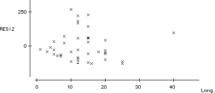
(e) elephant;

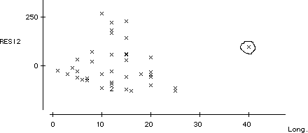
No, the elephant does not have the largest residual.

(f) giraffe; longer

(g) Gestation = 9.0 + 13.6 Longevity; 50.1%

(h) no

(i)

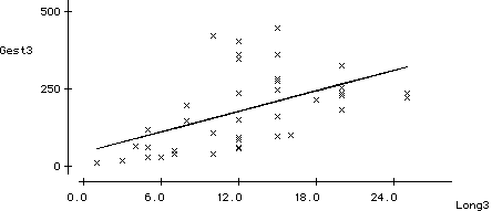
Gestation = 45.0 + 11.1 Longevity; 26.9%

(j) The removal of the elephant affected the graph more.

(k)

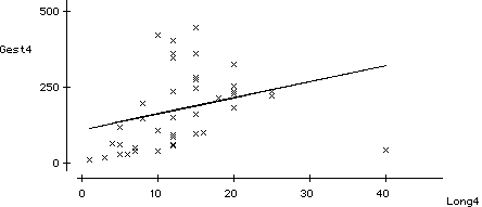
Gestation = 110 + 5.26Longevity
r^2 = .092

10-2: Planetary Measurements ( cont. )

(a) (Asks for interpretation)

(b) 0.910, a very strong, positive correlation which seems to indicate a strong linear relationship.

(c)

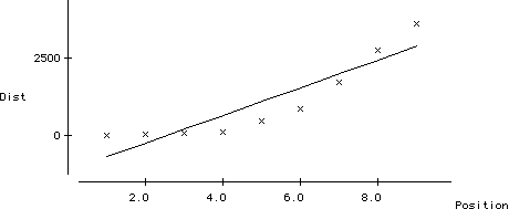
Distance = -1126 + 446 Position

(d) No, the line does not fit that data well. The line does not capture the curved aspect of the relationship.

(e)

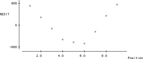
Yes, the residual plot reveals a clear, curved pattern.

10-3: Televisions and Life Expectancy ( cont. )

(a)

r = -0.804; the relationship does not appear to be linear

(b)

(c)

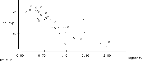
r = -0.855; the relationship appears to be stronger and more linear.

(d) life expectancy = 77.9 - 9.81Log(PerTV)

(e) 85.1%

(f) 55

(g)

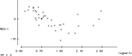
no

(h) The transformed data produces a better fit than the original data.

11-1: Penny Thoughts ( cont. )

(a)

(b)

11-2: Age and Political Ideology

(a) 0.205

(b) 0.388

(c) 0.406

(d) 0.280

(e) 0.473

(f) 0.247

(g)-(h)

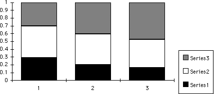
Series 1 - Liberal
Series 2 - Moderate
Series 3 - Conservative

(i) (Asks for interpretation)

(j) 0.473

(k) 0.199

(l) 0.097

11-3: Pregnancy, AZT, and HIV

(a) (Asks for prediction)

(b) AZT: 0.079; HIV: 0.250

(c) 3.23

(d) (Asks for interpretation)

11-4: Hypothetical Hospital Recovery Rates

(a) A: 0.8; B: 0.7; B saves the higher percentage.

(b) Are you convinced?

(c) A: 0.983; B: 0.967; A saves the higher percentage.

(d) A: 0.525; B: 0.3; A saves the higher percentage.

(e) Hospital A tends to treat the large majority of patients in "poor" condition. Since these patients are more likely to die than those in "fair" condition, A's overall survival rate is lower than B's despite being higher for each type of patient.

(f) Hospital A is preferable regardless of one's condition.

11-5: Hypothetical Employee Retention Predictions

(a) 0.16

(b) 0.16

(c) no

(d) no

(e)

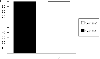
Series 1 - Predicted to stay
Series 2 - Predicted to leave

(f)

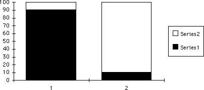
Series 1 - Predicted to stay
Series 2 - Predicted to leave