Workshop Statistics: Discovery with Data and Fathom
Topic 26: Inference for Two-Way Tables
Activity 26-1: Suitability for Politics (cont.)
(a) observational units = sample of American adults
variable 1: whether or not they agree with the statement; categorical
binary
variable 2: their political view: categorical
(b) Tend to have more agreement with statement as lean more conservative.
While there is definitely a trend it may not be all that strong.
(c) agreement proportion = 382/1685 = .227
(d) Liberals: 484(.227) =109.87
(e) Moderates: 610(.227)=138.47
Conservatives: 591(.227)=134.16
(f) 382(484)/1685=109.73
(g) rest of row is 138.47 and 134.16
(h) (74-109.87)2/109.87 = 11.632
(139-138.47)2/138.47 = .004
(169-134.16)2/134.16 =9.152
(410-374.27)2/374.27 =3.140
(471-471.71)2/471.71 = .001
(422-457.02)2/457.02 = 2.683
sum = 26.881
(i) large values of the test statisitc will be evidence against the
null hypothesis (indicate larger discrepancies between the observed and
the expected)
(j) df = (3-1)(2-1) = 2
26.881 is off the chart so p-value is < .0005
(k) It would be highly unusual to observe these sample data by chance
alone if there was independence between agreement and political leaning.
We have very strong evidence that political leaning is related to peoples
agree with the statement "Most men are better suited emotionally for politics
than are
most women."
Activity 26-2: Government Spending
(a) Ho: There is no association between opinionon spending and
political leaning
Ha: There is an association between opinionon spending and
political leaning
(b) 133(376)/1235 = 40.49
590(435)/1235 = 207.81
512(424)/1235 = 175.78
(c) (40.49-50)2/50 = 2.232
(214-207.81)2/207.81 = .184
(176-175.78)2/175.78 = .000
sum=6.724
(d) with df=(3-1)(3-1)=4, find .1 < p-value < .2
(e) There is no evidence of an association between opinion and spending
on space program.
Activity 26-3: Newspaper Reading (cont.)
(a)
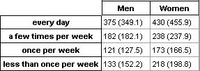
Ho: There is no association between gender and newspaper
reading
Ha: There is an association between gender and newspaper
reading
test statistic: 8.261, p-value = .041
We would reject the null hypothesis at the .05 level and conclude there
is a relationship between gender and newspaper reading. (We would not reject
at the .01 level.)
(b)
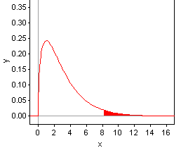
The shaded region represents the probability of
seeing a test statistic as large as the one observed (8.261) when there
is no association. Since this probability is small (less than .05)
we make conclude that there probably is some association between gender
and newspaper reading..
(c) The cell that corresponds to the male, reading less than once
per week contributes the most to the test statistic. The observed count
is lower than the expected count for that cell, meaning that there are
fewer males reading less than once per week than we wouldve expected if
there was no relationship.
(d) The next three cells are the cells that correspond to men reading
every day, women reading every day, and women reading less than once per
week. There are more men than we would have expected reading every
day, there are fewer women then we would expected reading every day and
more women
than expected reading less than once per week. Seems men read more
than women.
Activity 26-4: Suitability for Politics (cont.)
(a)
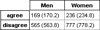
Ho: There is no association between gender and suitability
opinion
Ha: There is an association between gender and suitability
opinion
test statistic: .01776, p-value: .89
With our large p-value, there is no evidence of an association between
gender and their opinion on whether men are more suitable for politics
than women.
(b) Let q1=proportion
of men who agree with the statement and q2=proportion
of women who agree with the statement
Ho: q1=q2
(men
and women agree in equal proportions)
Ha: q1¹q2(the
proportions of men and women who agree differs)
test statistic: -.13, p-value: .894
Again, with this large p-value, we would fail to reject Ho:
q1=q2,
giving
us no evidence that men and women don't agree in the same proportion.
(c) The p-values are equal, and
the conclusion is the same.
(d) z=-.13, z2=.0169
which is close to .018.
Activity 26-5: Government Spending (cont.)
Answers will vary.
These are sample answers.
(b) Sample
output:
|
liberal |
moderate |
conservative |
total |
| too little |
45 |
43 |
45 |
133 |
| just right |
169 |
224 |
197 |
590 |
| too much |
162 |
168 |
182 |
512 |
| total |
376 |
435 |
424 |
1235 |
Chi-square
statistic for this table: 4.174
(c) This is
smaller than 6.724, the chi-square statistic from the actual sample data.
(d)
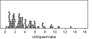
(e) There were
11 values in this graph larger than 6.725. This is 11% of the repetitions.
(f) Earlier
we found p-value to be between .1 and .2, and .11 is within this range,
so yes, we are reasonable close. They should match since the p-value
tells us how often we expect to get a chi-square value at least this extreme
when the null hypothesis is true.