Workshop Statistics: Discovery with Data and Fathom
Topic 23: More Inference Considerations
Activity 23-1: Racquet Spinning (cont.)
(a) (.362, .558)
(b) yes
(c) Based on our answer to (b), we would not expect a significance
test of whether q differs from .5 to be significant
at the .05 level because the interval indicates that .5 is a plausible
value for q.
(d) test
statistic = -.8
p-value
= .424
Since the p-value is so large, the
sample proportion does not differ significantly from one-half at the .05
significance level. So, yes, our expectation in (c) was realized.
(b)-(h)
|
Hypothesized value
|
Contained in 95% CI?
|
Test statistic
|
p-value
|
Significant at .05?
|
|
.35
|
no
|
2.31
|
.021
|
yes
|
|
.40
|
yes
|
1.22
|
.221
|
no
|
|
.50
|
yes
|
-.80
|
.424
|
no
|
|
.55
|
yes
|
-1.81
|
.070
|
no
|
|
.60
|
no
|
-2.86
|
.004
|
yes
|
(i) If the hypothesized value is contained in the 95% confidence interval,
it will not be significant at the .05 level, and vice versa.
Activity 23-2: Racquet Spinning (cont.)
(a) sample proportion: .565; test statistic: 1.84; p-value:
.066; significant at .05?: no
(b) sample proportion: .575; test statistic: 2.12; p-value:
.034; significant at .05?: yes
(c) sample proportion: .650; test statistic: 4.24; p-value:
.000; significant at .05?: yes
(d) a and b
(e) b and c
Activity 23-3: Cat Households (cont.)
(a) 99.9% confidence interval: (.268, .278); Hypotheses: Ho:
q
= .25, Ha: q > .25; test
statistic: 15.02; p-value: less than .0002 (.0000 to many decimal
places).
(b) Yes, because the entire 99.9% confidence interval is greater than
.25, and the test of significance reveals very strong evidence against
the null hypothesis that theta equals .25.
(c) No, it is most likely only 1-2% more than 25% since the 99.9% confidence
interval is only (.268, .278).
(d) confidence interval
Activity 23-4: Hypothetical Baseball Improvements
Students' answers to (a)-(g) may differ. These
are meant to be sample answers.
(a)
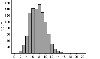
<------------number
of hits -------------->
This distribution is symmetrical,
with the center at 7. The spread is from 1 to 15.
(b) About 13, because 5% of the data points lie above this point.
(c)
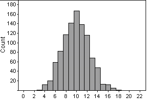
<------------number of hits
---------------->
The top distribution is using a .250 hitter, while the
bottom is using a .333 hitter. This distribution for the .333 hitter
is also symmetrical, with the center at 10. The spread is from 3
to 18. There is quite a bit of overlap between the two distributions.
(d) The .333 hitter exceeded 13 hits about 12 percent of the time.
(e) No. Even though he is actually a .333 hitter, there is only
about a 12% chance that he will get enough hits (>13) to convince us that
he's not a .250 hitter. Also, we know that since the overlap between
the two distributions is so great, most of the time a .333 hitter will
have a number of hits that could easily fall on the .250 hitter's distribution,
meaning it would bot be significantly better than a .250 hitter.
(f) Approximate power = .12
(g)
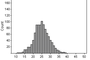
There is less overlap between the two distributions.
From the first distribution (that of a .250 hitter), he'd be in the top
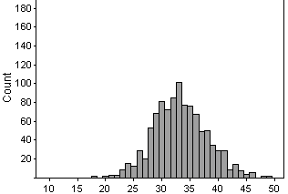
5% of performances if he got more than 34 hits or so. When he is a .333
hitter, he will get more than 34 hits almost 50% of the time. Thus, there
is a much higher chance that he will be able to convince us he is better
than a .250 hitter. Increasing the sample size gives us more evidence and
increases the power we have to detect that his performance has improved.
(h) more powerful (the distribution will now be centered higher and
have less overlap with .250 distribution), he's a much better hitter so
it's much easier for him to perform convincingly higher than a .250 hitter.
(i) more powerful. He doesn't need to perform as high to convince us
he has improved.
(j) alternative value, level of significance
Activity 23-5: Halloween Practices (cont.)
(a)1.96sqrt(.69(.31)/1005)= .0286
(b) We would need a larger sample because larger samples make the statistic
more accurate.
(c) Solve 1.96sqrt(.69(.31)/n)=.01 for n to find that n=8,218
(d) We would need even more people because increasing the confidence
without changing the margin or error would require a larger sample size.
(e) Solve 2.576sqrt(.69(.31)/1005) to find n=14,194
(f) The population size did not enter into these calculations at all.
The answers to (c) and (e) would be no different if the population of interest
were all California adults rather than all American adults.
(g) Every person in the population would have to be interviewed to
determine the value of the population proportion exactly, with 100% confidence.
Activity 23-6: Hypothetical ATM Withdrawals (cont.)
(a)
| |
Sample size
|
Sample mean
|
Sample std. dev.
|
95% confidence interval for m
|
|
machine 1
|
50
|
70
|
30.3
|
(61.39, 78.61)
|
|
machine 2
|
50
|
70
|
30.3
|
(61.39, 78.61)
|
|
machine 3
|
50
|
70
|
30.3
|
(61.39, 78.61)
|
(b)
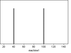
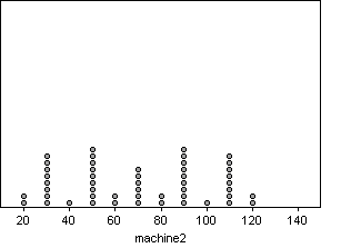
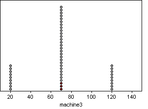
These distributions are
very different from each other. While many of their descriptive statistics,
such as sample size, mean, and standard deviation are the same, the distributions
still differ greatly.
Activity 23-7: Female Senators (cont.)
(a)( .034, .146)
(b) no
(c) The technical conditions necessary for this procedure to be valid
are not fully met. This sample is not a simple random sample from
the population of interest. The male/female ratio in the 1999 U.S.
Senate is not representative of all humans.
(d) The interval does not make sense for this purpose because we know
the population proportion of women to be .09 for the 1999 U.S. Senate.