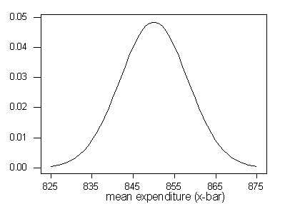
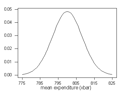
Students' answers to (a)-(n) may differ since the data is chosen randomly. These are meant to be sample answers.
(b)
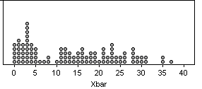
Yes, this resembles the distribution of ages in the population.
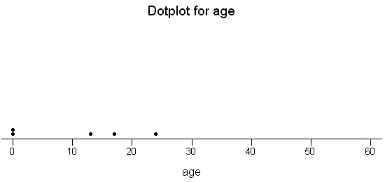
|
|
|
|
|
|
|
|
|
|
|
|
|
|
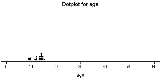
Students' answers to (a)-(n) may differ since
the data is chosen randomly. These are meant to be sample answers.
(b)

Yes, this resembles the
distribution of ages in the population.
(c)-(i)
|
m = 12.264 |
s = 9.613 |
|
|
|
size |
|
|
|
|
|
|
|
|
|
|
|
|
|
|
|
|
|
|
|
|
|
|
|
(c) The sample mean of 13.76 and the sample std.dev.
of 10.314 are reasonably close to their population counterparts.
The distribution is skewed to the right, with a peak at 3 years old.
(d)
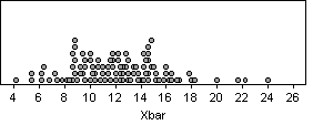
This distribution is much
more symmetric (much less skewed to the right) then either the population
distribution or the distribution attained with only a sample size of 1
for each mean. Also, this distribution has a much smaller spread.
(e) The sample mean (12.238) is very close to the actual population
mean, while the sample standard deviation of 3.659 is much lower than the
actual population standard deviation of 9.613. The distribution is
much more symmetric (not skewed to the right nearly as much as the population
distribution).
(f)
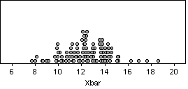
This distribution is more
normally shaped than either the population distribution or the distributions
from using sample sizes of 1 and 5. It is also a narrowed distribution
(less spread).
(g) Once again, the sample mean is close to the population mean, and
the sample standard deviation is much lower than the population standard
deviation. This sample standard deviation is even lower than the
sample standard deviation when using a sample size of 5. The shape
of the distribution does not resemble the population distribution at all.
This distribution is normally shaped, while the population distribution
was skewed to the right.
(h)
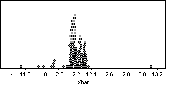
This distribution is much more localized than either the population distribution
or the distributions from the sample sizes 1, 5, and 25. Like the
sample size of 25 (unlike the population distribution or the sample size
of 1), it appears to be normally distributed, but with a very narrow spread.
(i) The sample mean is very close to the population mean (and
the sample means from the distributions using all the other sample sizes).
However, the sample standard deviation is MUCH smaller than the population
standard deviation. The distribution is much more localized around
the mean (less spread out), and distributed normally as opposed to being
skewed to the right.
(j) Although answers may vary, the correct answer is yes (neither
of the populations has a distribution that is close to normal).
(l)
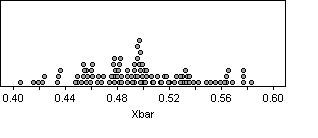
This appears to be a normal
distribution.
(m)
|
|
|
|
|
|
|
|
|
|
|
|
|
|
|
|
|
|
|
|
|
|
|
|
|
(m) The sample mean is close to the population mean, while the sample
standard deviation is much smaller than the population's.
(n) (l)
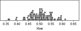
This also appears to be
a normal distribution.
(m) Once again, the sample mean is close to the population
mean, while the sample standard deviation is much smaller than the population
standard deviation.
(o) Penny ages: 1.359; 1: .041; 2: .050; these are reasonably
close to the values we obtained for the standard deviation of the 100 simulated
sample means.
