Workshop Statistics: Discovery with Data, Second
Edition
Topic 27: Inference for Correlation and Regression
Activity 27-1: Baseball Payrolls
(a) There appears to be a moderate positive association between payroll
and winning percentage.
(b)
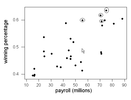
These teams seem to have large payrolls and larger winning percentages.
(c) Positive relationship with moderate strength. Student
guesses will vary.
Actual r=.630
(d) Answers will vary. These are intended to
be sample answers.
Below is one possible random assignment.
| payroll |
win pct |
| 70.3710 |
0.598765 |
| 75.0650 |
0.444444 |
| 55.3685 |
0.475309 |
| 42.1428 |
0.588957 |
| 54.3925 |
0.395062 |
| 15.1500 |
0.635802 |
| 55.5640 |
0.456790 |
| 71.1358 |
0.413580 |
| 42.9274 |
0.419753 |
| 16.3630 |
0.530864 |
| 71.3314 |
0.617284 |
| 30.5165 |
0.595092 |
| 24.2177 |
0.484472 |
| 46.2482 |
0.475309 |
| 45.9322 |
0.459627 |
| 46.0096 |
0.465839 |
The correlation coefficient for these two columns is r=-.281
(e) This correlation is not nearly as large as the one observed in
the sample (.630).
(f)
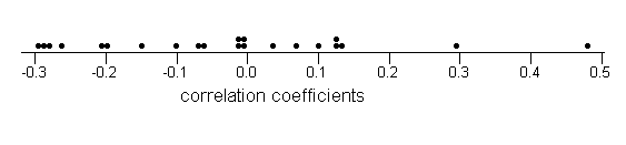
(g) The graph is fairly symmetric, centered around zero.
(h) None is close to the correlation we observed in the sample and
thus the sample correlation (.705) is very unlikely to happen by chance
alone, indicating that the relationship between winning percentage and
payroll is statistically significant.
(i) t = .630 sqrt(16-1)/sqrt(1-.6302) = 3.03 with 16-2=14
degrees of freedom.
Table III indicates that .001 < one-sided p-value <
.005
With such a small p-value, we have strong evidence against the null
hypothesis of no association, suggesting that there is an association between
payroll and winning percentage.
Activity 27-2: Studying and Grades
(a) observational units: students surveyed
variable 1: hours of study (quantitative)
variable 2: GPA (quantitative)
(b)
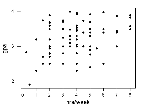
There appears to be a fairly weak positive association between hours
studied per week and gpa.
(c) Predicted gpa= 2.89 + .0894 hours/week
correlation coefficient, r=.343
(d) the slope=.0894 indicates the change in gpa for an increase of
one study hours/week.
(e) no, sampling variability
(f) correlation and regression slope are both essentially zero.
Answers will vary, these are intended as sample
answers.
Note: the answers to (g)-(s) below are the answers
to (h)-(t) in the Minitab version.
(g) bs
-0.0245873 0.0126319
-0.0007703 0.0307915 -0.0238198 -0.0216128
-0.0191908 0.0065811
-0.0245659 -0.0283816 0.0386437 -0.0215482
-0.0247520 0.0427848
0.0099658 0.0094685 0.0041925 -0.0075949
-0.0114600 -0.0241534
(h)
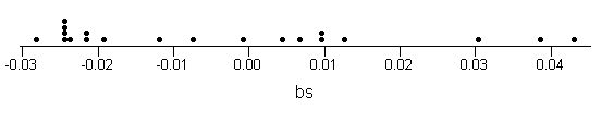
(i) .0894 is nowhere near any of these values. This indicates that
the sample result of .0894 is extremely unlikely to occur by chance alone.
(j) mean close to zero, standard deviation: .0225
(k) For sample data, the standard error of the slope coefficients is:.02771.
This is close to .0225.
(l) t=.0894/.02771 = 3.23 with df=80-2=78.
(m) Using df=80, we'd get a .0005< p-value<.001
(n) This small p-value is consistent with the simulation results which
never had a sample slope above .045.
(o)Yes
(p) t*(n-2)=1.990
b + 1.990 (.0225) = (.045,.134)
(q) We are 95% confident that the increase in GPA for an additional
hour of study time is between .045 and .134
(r)
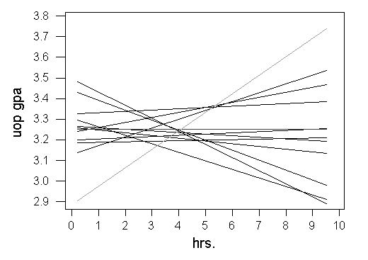
The sample line appears quite different from the simulated lines.
(s) Thus a slope this extreme is not very likely to occur if there
is no relationship between the two variables in the population. This indicates
that we have strong evidence of an association between hours of study and
gpa.
Activity 27-3: Studying and Grades (cont.)
(a)-(b)
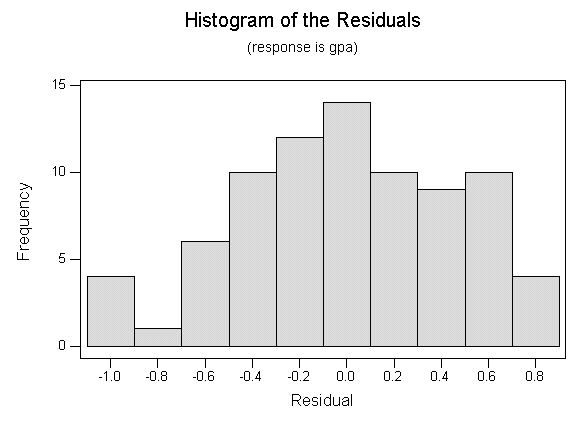
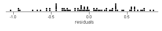
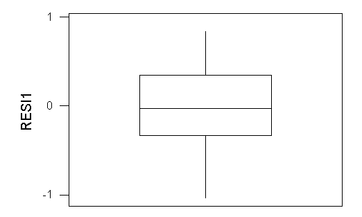
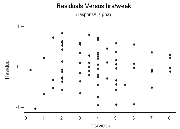
The residuals plot look reasonably symmetric and normal. I would consider
the normality condition met.
The residuals vs. hrs/week does not seem to show a strong nonlinear
pattern. The variability in the residuals is also relative constant
(expect maybe at the high hrs/week end, but we don't have many observations
there.