Workshop Statistics: Discovery with Data, Second
Edition
Topic 25: Comparing Two Means
Activity 25-1: Sentence Lengths (cont.)
(a)There is a typo in this problem, the standard
deviation for Moore should be 6.42 not 15.58.

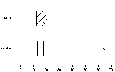
(b) Grisham has a wider distribution of words per sentence. He
also has a higher mean, min, max, and IQR.
(c) yes
(d) Ho: mG = mM
Ha: mG ¹mM
(e) using s(moore)=15.58 t = 1.43
using s(moore)=6.42,
t=1.93
(f) df=min(27,39)=27, area above 1.93 is between .025 and .05 so two-sided
p-value is between .05 and .1
(g) The p-value is the probability of getting sample data so extreme
if in fact Grisham and Moore have the same mean number of words per sentence
in these books.
(h) no
(i) no
(j) 1. That the two samples are independently selected simple random
samples from the populations of interest. 2. Either that both sample
sizes are large (n1 > 30 and n2 > 30
as a rule of thumb or that both populations are normally distributed. We
do have a large outlier in the Moore data, but the sample sizes are reasonable
large. Looking at dotplots you could decide if the samples look reasonably
normal. These are also sentences from chapter 3, not from the entire book,
or all of the author's writings. However, it would be good to be
cautious with these results.
Activity 25-2: Hypothetical Commuting Times
(a) no
(b) Route 1 seems to be quicker.
(c)
| |
sample size
|
sample mean
|
sample std. dev.
|
|
Alex route 1
|
10
|
28
|
6
|
|
Alex route 2
|
10
|
32
|
6
|
(d) p-value: .155
(e) Alex's sample results are not statistically significant at any
of the commonly used significance levels, so he cannot reasonably conclude
that one route is faster than the other for getting to work.
(f) (-8.67, 0.67)
(g) Yes, this interval contains zero. This means that (within
90% confidence) zero is a plausible value for the difference in Alex's
mean commuting times for these two routes.
(h) Barb's route 1 times differ from her route 2 times more greatly
than Alex's.
(i) Carl's times are very concentrated, while Alex's are much more
varied.
(j) Donna has many more data points than Alex.
(k)
| |
sample size
|
sample mean
|
sample std. dev.
|
p-value
|
|
Barb route 1
|
10
|
25
|
6
|
.002
|
|
Barb route 2
|
10
|
35
|
6
|
|
|
Carl route 1
|
10
|
28
|
3
|
.008
|
|
Carl route 2
|
10
|
32
|
3
|
|
|
Donna route 1
|
40
|
28
|
6
|
.004
|
|
Donna route 2
|
40
|
32
|
5.995
|
|
(l) Barb: The times between route 1 and route 2 differed much more
than Alex's.
Carl: Carl's times had half the sample std.
dev. that Alex's did.
Donna: Donna had 4 times the sample size as
Alex.
Activity 25-3: Children's Television Viewing (cont)
(a) No, if the randomization achieved its goal, the children would be as
similar as possible prior to the curriculum intervention.
(b) Ho: mctrl = mintv
(there is no difference in the mean number hour per week spent viewing
television between the control and treatment groups)
Ha: mctrl ¹mintv
(there is a difference)
(c) t = .055
(d) p-value > .2
(e) no
(f) Ho: mctrl = mintv
Ha: mctrl > mintv
t = 3.27;
.001 > p-value > .0005
We would reject the null hypothesis at the .05 level.
(g) Notice that the std. devs. are nearly as large, in one case larger,
than the means. Since negative values are impossible here, it cannot
be the case that the distributions are symmetric with 68% falling within
one standard deviation of the mean and 95% within two. Thus, the
distributions cannot be normal, but skewed to the right instead.
(h) The nonnormality of these distributions does not hinder the validity
of using this test procedure because both samples have n > 30.
(i) Before the study, the two groups were similar in terms of television
viewing. After the study, the intervention group had significantly
decreased their television viewing time. We would conclude that the
curriculum intervention succeeded in reducing television viewing.
Randomization served to make the groups similar in regards to television
viewing prior to the imposition of the treatment, so that the differences
observed after the experiment could reasonably be attributed to that treatment.
