Workshop Statistics: Discovery with Data, Second Edition

Topic 22: Tests of Significance II: Means

Activity 22-1: Basketball Scoring

(a) m = 183.2 (null hypothesis)
(b) m > 183.2 (alternative hypothesis)
(c)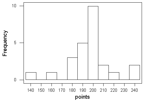

The distribution looks pretty symmetric, though has some outliers on both ends. Many of the observations fall above 183.2 points. This indicates some
evidence of an increase in the points per game scored after the rule change.
(d) sample mean,

= 195.88; sample standard deviation, s=20.27
(e) yes
(f) yes, sampling variability

Activity 22-2: Basketball Scoring (cont.)

(a) H_o: m = 183.2 ; H_a: m > 183.2
(b) t=3.12
(c)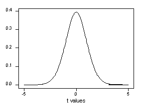

I’ve shaded above 3.13. Note, this shaded region is not very big, so I expect the probability I calculate to be rather small.
(d) The area to the right of our test statistic is between .001 and .005.
(e) The p-value tells us that there is between a .1% and .5% chance that we’d get a sample mean this big (>195.88) if there was no improvement in scoring
after the rule changes.
(f) We would reject the null hypothesis at a levels of .10, .05, .01, and .005. Even though we don’t know the p-value exactly, we know it’s smaller than these
values.
Note: The answers to (g) and (h) below are the answers to (h) and (i), respectively, in the Calculator version.
(g) First, we would’ve needed a simple random sample of games from this season. We didn’t have that, but it might be reasonable to assume that games
midseason are fairly representative. Second, since our sample size is less than 30, we would need to know the population of points per game follow a normal
distribution. We can’t verify that, but the sample looks reasonably normal.
(h) The sample data does provide evidence that the mean points per game in the 1999-2000 season is higher than in the previous season. Still, we must be very cautious in this conclusion since the technical conditions are not exactly met (e.g. maybe scores tend to be higher in December).

Activity 22-3: Sleeping Times (cont.)

Results will vary depending on class results, but the set up is:
(a) Let m=average sleep time of all students at the school
H₀: m=7 (get 7 hours on average)
H_a: m<7 (is there evidence of less than 7 hrs)
(b) technical conditions
Do you think students from your class are representative of students from the whole school? Would be questionable if it is a morning class.
If sample size of class is greater than 30, the normality condition will be considered satisfied.
(c) Sample 1 supplies stronger evidence that m < 7 because it has a smaller standard deviation.
(d) Sample 3 supplies stronger evidence that m < 7 because it has a larger sample size.
(e)

Sample number	Sample size	Sample mean	Sample std. dev.	p-value
1	10	6.6	.825	.080
2	10	6.6	1.597	.224
3	30	6.6	.825	.006
4	30	6.6	1.597	.090

(f) sample 3
(g) Our conjectures in (c) and (d) are correct.

Activity 22-4: Marriage Ages (cont.)

(a) The differences, in order, are: 3, -7, 1, 0, 5, 3, 15, 7, 1, 10, 0, -5, 1, 1, 3, -2, -1, -5, 2, 2, 3, 8, 1, -1
(b)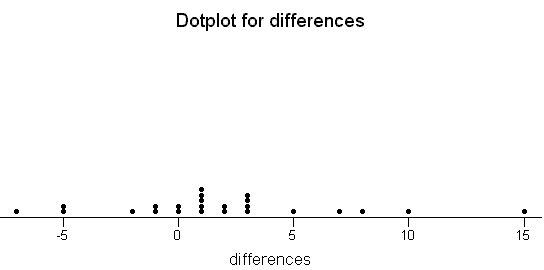

(c)

= 1.875; s = 4.812; n = 24
(d) The parameter of interest is m=the mean difference in ages at the time of a Cumberland County, PA couple's marriage (husband - wife).
H_o: m = 0 (no age difference on average)
H_a: m > 0 (husbands tend to be older on average)

n is not greater than 30 but the sample of differences looks reasonably normal. We are considering these couples a simple random sample of couples in Cumberland County, PA, in 1993.
        t = 1.90
        23 degrees of freedom
        The area to the right of the t-statistic is between .025 and .05, which suggests moderately strong evidence against H_o.
The p-value is less than .05. Therefore we reject H_o and conclude that there is significant evidence that husbands tend to be older on average in this population.
(e) (0.191, 3.558); This interval does not include zero. Again, must consider the technical conditions.
(f) There is enough evidence to reject the null hypothesis that m = 0, as long as the sample was random and the population differences comes from a normal distribution. If so, have statistically significant evidence that men are older. The confidence interval indicates that this mean age difference is between .19 years and 3.6 years.