Workshop Statistics: Discovery with Data, Second
Edition
Topic 18: Central Limit Theorem
Activity 18-1: Smoking Rates
(a) q
(b) Not necessarily due to sampling variabilty.
(c) The CLT says that this sample proportion should have a normal distribution,
with mean equal to q=.229, and standard deviation
equal to sqrt(q(1-q)/n)
= sqrt(.229*.771/100) = .042.
(d) Shade .25 and above. Guesses will vary from student to student.
(e) mean of sampling distribution: .229; standard deviation of
sampling distribution: .042; z-score standardizing .25 = (.25-.229)/.042
= .5
(f) probability  above
.5 = 1-.6915= .3085
(g) The sampling distribution based on a larger sample size will still
be centered at .25, but will exhibit less variability: sqrt(.229(1-.229)/400)=.021.
We expect these  values to fall closer to .229, so the probability of a sample result above
.25 would be smaller.
(h) z=(.25-.229)/.021 = 1.00, proportion above = 1-.8413 = .1587
(i) Variabilty will decrease and a sample proportion above .25 will
be even less likely. z=(.25-.229)/sqrt(.229(1-.229)/1600) = 2, proportion
above = 1-.9772= .0228
(j) no
(k) There would be no changes.
Activity 18-2: Smoking Rates (cont.)
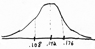
(a) SD=sqrt(.142(1-.142)/100)=.035

<-----------------  values ----------------->
(b) mean=.142, sd=.035
z=(.25-.142)/.035 = 3.09
proportion above = .001
So P( >.25) =
.001
(c) The standard deviation will decrease, which increases the z-score,
which decreases the probability that the sample proportion would exceed
.25.
(d) We would have strong reason to doubt that the state was Utah because
there is such a small probability (.001) of there being any more than 25
smokers in a sample of 100 Utah residents that it would be hard to believe
that a random sample of 100 Utah residents would yield 25 smokers.
Activity 18-3: Candy Bar Weights (cont.)
(a) Want P(2.18 <  <
2.22) where xbar follows a normal distribution with mean m=2.20
and standard devaition s=.04
Z(2.18) = (2.18-2.20)/.04 = -.5
proportion below -.5 = .3085
Z(2.22) = (2.22-2.20)/.04 = .5
proportion below .5 = .6915
Subtracting to find the area between = .6915-.3085 = .3830
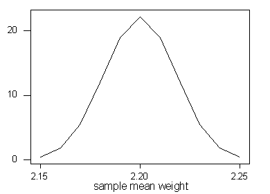
(b) These sample means will have a normal distribution, centered at
m=2.20,
but now with standard deviation s/sqrt(5)=.04/sqrt(5)
=.018

(c) shading
(d) The z-scores are (2.18-2.20)/.018 = -1.11 and (2.22-2.20)/.018
= 1.11, so the probability that the average weight of 5 candy bars will
be between 2.18 and 2.22 ounces is .8665-.1335 = .7330.
(e) The probability will increase if the sample size were 40 instead
of 5 because the standard deviation will decrease and the values will be
more concentrated around 2.20, so there will be a greater concentration
of sample mean values in this middle range between 2.18 and 2.22.
(f) The standard deviation of the sample means is now sigma/sqrt(n)
= .04/sqrt(40) = .0063. The z-scores are (2.18-2.20)/.0063 = -3.17
and (2.22-2.20)/.0063 = 3.17, so the probability that the average weight
of 40 candy bars will be between 2.18 and 2.22 ounces is .9992-.0008 =
.9984
(g) The calculations in (f) would remain approximately correct even
if the candy bar weights themselves had a skewed, nonnormal distribution
since the Central Limit Theorem establishes that the distribution of sample
means will be approximately normal distribution for a sample size as large
as n = 40. The normal approximation would not be valid with
n
= 1 or n = 4.
Activity 18-4: Candy Bar Weights (cont.)
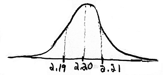
(a) SD( )=.04/sqrt(60)=.00516
Z(2.19)=(2.19-2.20)/.00516 = -1.94, proportion below -1.94 = .0262
Z(2.21) =1.94, proportion below = .9738
probability of an  value beween 2.19 and 2.21 = .9476

<-------------  values ------------------->
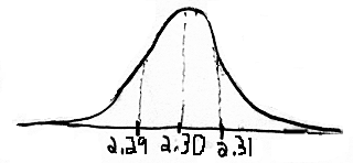
(b) The z-scores are the same as in (a), so the probability remains
.9476.

<-------------  values ------------------->
(c) They are equal.
(d) .9476, becuase the difference between the observation and the population
mean is still + .01, and the standard deviation does not change.
(e) There is a very high probability (.9476) that a sample of size
60 would result in a sample mean weight within + .01 of the actual
population mean.
Activity 18-5: Solitaire (cont.)
(a) std dev( ) =
sqrt(1/9(8/9)/10) = .099
z = (.10-1/9)/.099 = -.1122
proportion below = .4562
P( <.10) =
.4562
(b) .3079+.3849 = .6928 (Note: the probability of zero wins is .3079,
not .0379 as appeared in some printings of the book.)
(c) These are not at all close.
(d) The CLT provides a poor approximation for each probability in this
situation because the technical conditions concerning n and q
needed for the validity of the CLT are not met. n*q
is only 1.11, which is not greater than or equal to 10. n(1-q)
is only 8.88, which is not greater than or equal to 10.
