rStat 414 – Review 2 problem solutions
1) Consider this paragraph: The multilevel models we have considered up to this point control for clustering, and allow us to quantify the extent of dependency and to investigate whether the effects of level 1 variables vary across these clusters.
(a) I have underlined 3 components, explain in detail what each of these components means in the multilevel model.
Control for clustering: We have observations that fall into natural groups and we don’t want to treat the observations within the groups as independent, by including the “clustering variable” in the model, the other slope coefficients will be “adjusted” or “controlled” for that clustering variable (whether we treat it as fixed or random)
Quantify the extent of the dependency: The ICC measures how correlated the observations in the same group
Whether the effects of level 1 variables vary across the clusters: random slopes
(b) The multilevel model in the paragraph does not account for “contextual effects.” What is meant by that?
The ability to include Level 2 variables, variables explaining differences among the clusters. In particular, we can aggregate level one variables to be at Level 2 (e.g., group means).
(c) Give a short rule in your own words describing when an
interpretation of an estimated coefficient should “hold constant” another
covariate or “set to 0” that covariate
We should hold constant variable 2 when we are interpreting variable 1, unless the interaction of these two variables is also included, then if the other is at zero we can interpret the main effect of the first.
2) The article you read for HW 5 had the following: “application of multilevel models for clustered data has attractive features: (a) the correction of underestimation of standard errors, (b) the examination of the cross-level interaction, (c) the elimination of concerns about aggregation bias, and (d) the estimation of the variability of coefficients at the cluster level.
Explain each of these components to a non-statistician.
(a) Assuming independence allows us to think we have a larger sample size (more information) than we really do and underestimates standard errors.
(b) Including interaction terms between Level 1 and Level 2 variables
(c) Still get to analyze the data at Level 1 vs. aggregating the variables to Level 2 which could have a different relationship than the Level 1 relationship
(d) We are able to estimate the intercept-to-intercept and slope-to-slope variation at Level 2
3) (a)
Identify the three-levels in this study.
Level 1 = time point
Level 2 = plant
Level 3 = pot
The treatments were applied to the plots,
so they are Level 3 variables. Time is a
level 1 variable.
(b) Examine spaghetti plots of the plant heights
across the measurements for each of the species (coneflower and
leadplant). Is it reasonable to assume
linear growth between Day 13 and Day 28?
Does the initial height and/or rate of growth seem to differ between the
species? Is there more variability in
one species than the other?
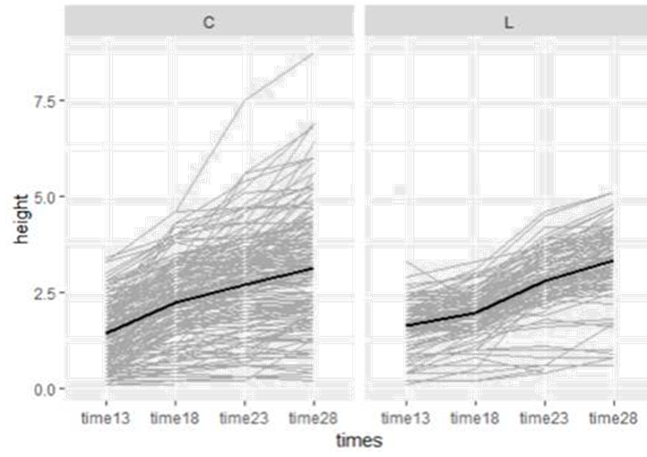
Linear growth seems a reasonable approximation. The initial heights
at time 13 and the overall slope from time13 to time 28 looks similar between
the two species but much more plant to plant variation for the coneflowers.
Maybe some evidence that coneflowers grow faster days 13 -18 and then slow
down, with leadplants catch up at the end.
(c) Examine spaghetti plots of the plant
heights over time separately for the three types of soil, separately for each
species. What do you learn?
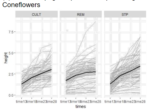
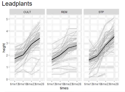
The rate of growth looks faster for Cult and Stp soils,
especially for the leadplants. Again more variation with the
coneflowers.
(d) Examine spaghetti plots of the plant
heights over time separately for the two levels of sterilization, separately
for each species. What do you learn?
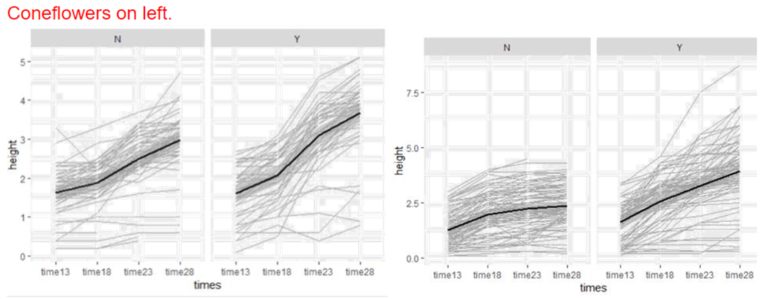
The rate of growth is faster for the sterilized plants and the non-sterilized coneflowers did better – there is little growth for the non-sterilized leadplants. Here I also see higher initial growth (day13) for the coneflowers.
Focusing on just the leadplants
(e) I next calculated time13 = time – time
13. Give two reasons this could be a
good idea.
If we were to include any
interactions or quadratic terms, this would guard against multicollinearity. It also makes the intercept of the model
correspond to the first time point.
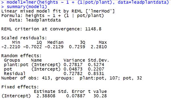
(f) Then I fit an “unconditional means” or
“random intercepts” model with no predictors.
How many parameters are
estimated? Provide an interpretation of each, including the variance
components. Anything interesting about the relative size of the variance
components?
We have estimated 4 parameters.
The intercept (2.388 in mm) estimates the overall average growth of
the plants on day 13 (average plant,
average pot)
The plant variance component (0.28) is a measure in the plant to plant variation in day 13 heights within the same
pot.
The pot variance (0.05) is a measure of the pot to
pot variation in day 13 heights.
The residual variance (0.73) is the variability of the plant heights
across the 4 time measurements within the same plant.
Total variance = .278 + .0487 + .7278 = 1.05
69% of the total variation is due to difference over time for each
plant, 26.4% is due to variability in the plants in the same pot, and only 4.6%
is pot to pot variation.
(g) Next I included the new time variable in the model assuming linear growth.
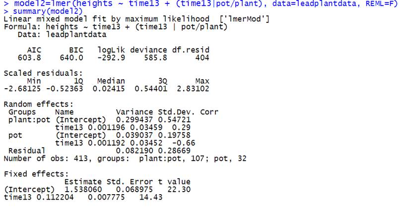
Explain what (time13|pot/plant) means to the
model. Write out the theoretical level equations (in terms of
![]() ’s). How many variance/covariance parameters are there/why?
’s). How many variance/covariance parameters are there/why?
How much of the within-plant variability is
explained by the linear changes over time?
Interpret the fixed effects. Are either of
the fixed effects statistically significant?
The (time13 | pot/plant) component is indicating that plants are
nested within pots and that we are allowing the growth rate (slope of time) to
vary across the plants and across the pots (as well as the intercepts =
measurement on day 13).
Let ijk refer to the ith measurement of the
jth
plant in the kth pot
Level 1 equation: ![]()
Level 2 equations: ![]() and
and ![]()
Level 3 equations: ![]() and
and ![]()
The composite equation can then be written as
![]()
where we have random variation in the intercepts at both Levels 2 and 3
and random variation in the slopes at both Levels 2 and 3.
There are 5 variance parameters
(within plant variation, between plant variation in intercepts, between plant
variation in slopes, between pot variation in intercepts, between pot variation
in slopes). There are 2 covariance parameters:
intercepts and slopes at level 2, intercepts and slopes at level 3. There are also 2
fixed parameters for 9 parameters total.
The within plant variability decreased from 0.7278 to 0.0822, an 89%
decrease! In other words 89% of the within plant variation in heights can be
explained by the linear growth over time.
The overall leadplant height for day 13 is 1.54mm, with an average
increase of 0.112 per day for an average plant in an average pot.
Both the intercept (initial plant height) and the slope are
statistically significant with t-ratios of 22 and 14 respectively.
(h) Next I added the sterilization and soil type variables, including
interactions with the time variable.

Why did I include interactions with the time
variable? Is this model a significant improvement from the model in (g)?
The interactions with time is
what puts the level 2 variable into the equation for
the random slopes. For example
![]()
corresponds to having a sterile x time term in the model.
![]()
Level 1 equation: ![]()
Level 2 equations: ![]() and
and ![]()
Level 3 equations: ![]()
and ![]()
This model estimates 15 parameters.
(i) But this model in running into some
boundary conditions. One option is to simplify the model, e.g., removing some
variance components. Write out the model
equations, for a new model so that the intercepts have random components at
Levels 2 and 3 but the slopes are only allowed to vary at level 2. What is
the practical interpretation of this modelling choice? How many parameters does this remove from the model?
[If you check, this model should be more
stable, and not significantly worse.]
Level 1 equation: ![]()
Level 2 equations: ![]() and
and ![]()
Level 3 equations: ![]()
and ![]()
Composite equation:
![]()
![]()
This model allows the growth rates to differ from plant to plant but
not from pot to pot (after accounting for soil type and sterilization).
This doesn’t change the fixed effects but
now there are only 5 variance components to estimate (2 fewer).
To run this model in R, you would use something like (time13 | plant)
+ (1 | pot), intercepts and slopes vary across plants
but only intercepts vary across pots.
(j) Next we could consider adding an interaction between sterilization and soil
type to the model, along with the three-way interaction between sterilization, soil
type, and time.
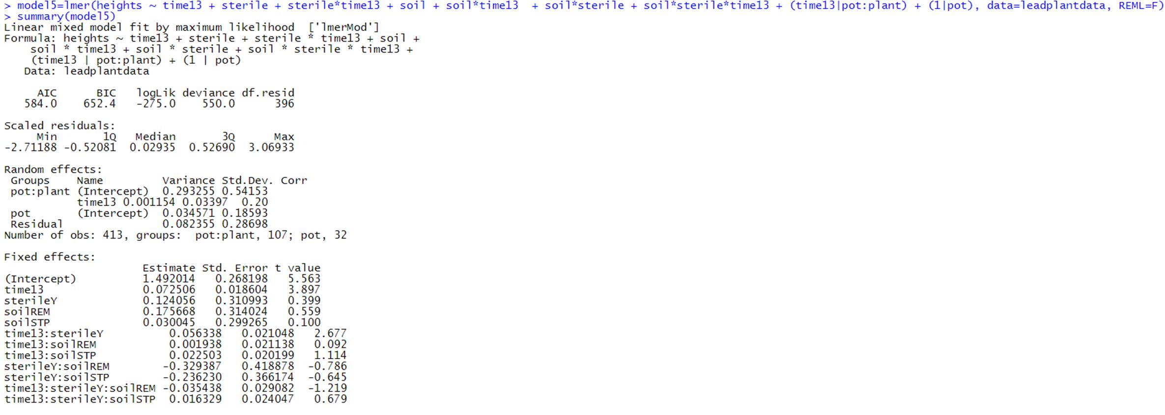
How many parameters does this add? Interpret
the nature of the three-way interactions. Explain what type of visual would
help you assess the evidence of such an interaction.
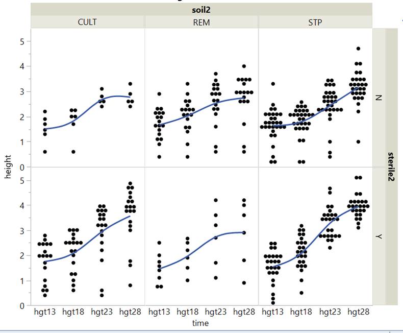
This adds 4 parameters to the model. We could look at a graph
of the plant heights over time vs. soil type with separate panels for
sterilized or not. This would allow us
to assess whether the change in growth rate across soil types is different
depending on whether or not the plants have been sterilized. In other
words, are the differences in the growth rates depending on type of soil type
differ for the sterilized or non-sterilized plants.
In the graph below, we see that the growth rates (slopes of the
line) appear similar across the three soil types for the non-sterilized plants.
For the sterilized plants, the growth rate looks a bit smaller for the REM
plants compared to CULT and STP. This three-way interaction ends up not being
statistically significant.
(k) How would you change the previous model so that neither
sterilization or soil type (or their interaction) are allowed
to influence Day 13 measurements? Why
might this be a reasonable consideration?
We would drop sterile, soilREM, and soilSTP and the 2 interaction
terms from the model. The first level 3 equation would become:
![]() ,but the second one
would not change. In other words, we would be forcing the (overall) fitted
model to start in the same spot in the 6 graphs above.
,but the second one
would not change. In other words, we would be forcing the (overall) fitted
model to start in the same spot in the 6 graphs above.
We saw in our exploratory data analysis that there didn’t seem to be much overall difference in the initial
heights across these treatments (maybe it takes two weeks for the effects of
these treatments to kick in). This is also supported by the small t-values for these 5 terms (remember if
your focus is on model building, you might want to create tet and validation datasets…)
(l) Return to the model in (j). Interpret
it! (A brief summary of the important features, especially as the agree/disagree with your exploratory data analysis. What
would the “effects plots” look like? What seems to maximize growth?!)
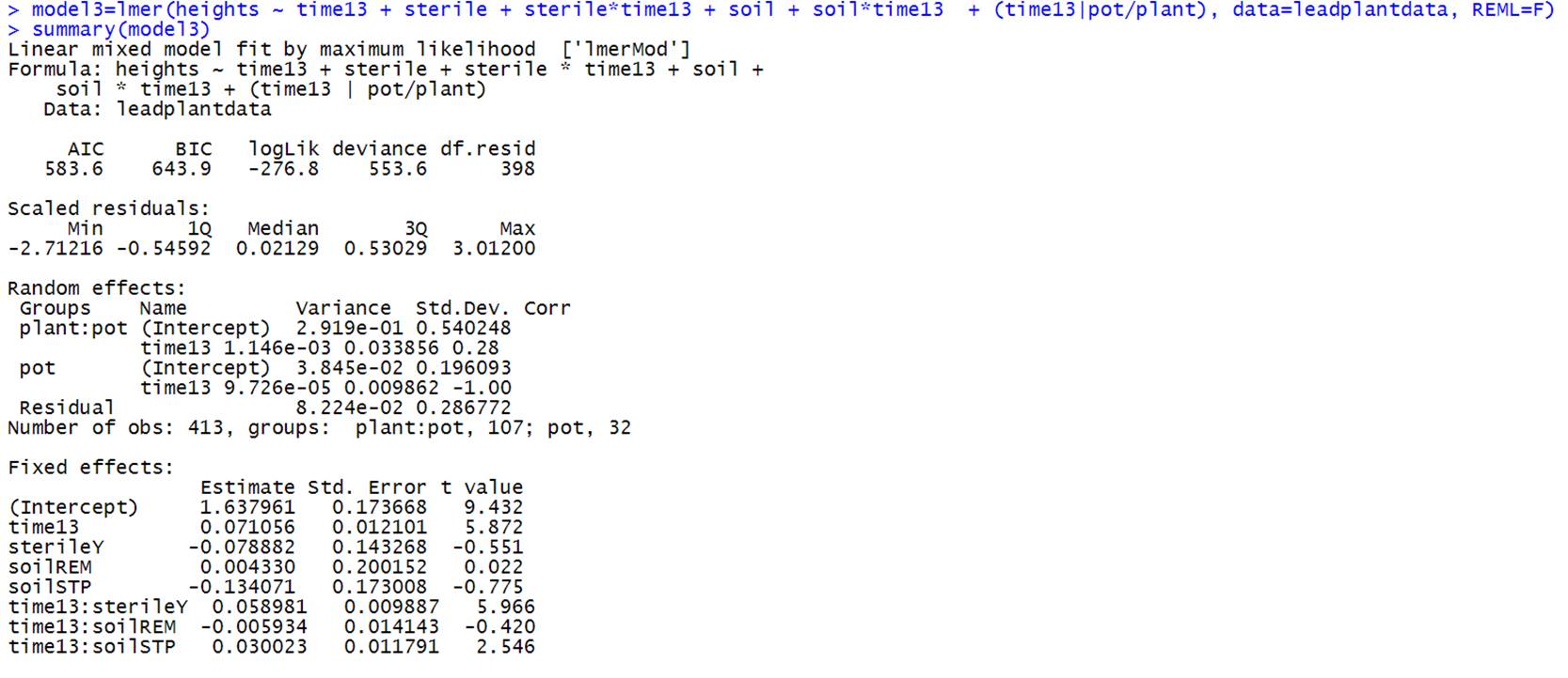
Focusing
on the significant treatments: Sterilizing the plants does not appear to have a
significant effect on day 13 height (t = -.551) but does appear to improve
their growth rate (t = 5.966), after adjusting for soil type but soil type doesn’t appear to make much of a difference. Restored (STP) soil appears to increase growth rate over
cultivated soil (t = 2.546) (don’t really have to talk about holding
sterilization fixed or picking a category in this factorial design (so no
confounding) with no 3-way interaction (so effect doesn’t change).
From
the later model, there is also weak evidence of an interaction, with sterilized
remnant soil having smaller growth rates (i.e., the benefit of sterilization is
somewhat muted in the remnant soil). So to maximize
growth, use sterilized (STP) soil.