Stat 414 – Review 2 problems

1) Consider this paragraph: The multilevel models we have considered up to this point control for clustering, and allow us to quantify the extent of dependency and to investigate whether the effects of level 1 variables vary across these clusters.

(a) I have underlined 3 components, explain in detail what each of these components means in the multilevel model.

(b) The multilevel model in the paragraph does not account for “contextual effects.” What is meant by that?

(c) Give a short rule in your own words describing when an interpretation of an estimated coefficient should “hold constant” another covariate or “set to 0” that covariate

2) The article you read for HW 5 had the following: “application of multilevel models for clustered data has attractive features: (a) the correction of underestimation of standard errors, (b) the examination of the cross-level interaction, (c) the elimination of concerns about aggregation bias, and (d) the estimation of the variability of coefficients at the cluster level.

Explain each of these components to a non-statistician.

3) Large scale alteration (e.g., destruction) of native prairie communities has been associated with numerous problems (e.g., soil erosion, lack of biodiversity of plants, increase in atmospheric CO₂). This has led to an increase in prairie reconstruction projects, but there has been a lot of variability in the success of these projects, even those using the same seed combinations and dispersal techniques in different years. A 3x2x2 factorial design was conducted to investigate the impact of soil type (remnant, cultivated, restored), sterilization (yes or no), and species (leadplant and cornflower) on the height on germinating plants. Each of the 12 treatments was replicated in 6 pots, for a total of 72 pots. Six seeds were planted in each pot. (OK, a few pots had more than six plants, probably because two of the microscopically small seeds stuck together when planted.) Measurements on each plant in each pot were taken at 13, 18, 23, and 28 days after planting. Plants that did not germinate are removed from the analysis (so we will restrict our study conclusions to plants that germinate!). Not all plants survived to the end of the 28^th day.

(a) Identify the three-levels in this study. Also identify any Level 2 or Level 3 variables in the study.

Step 0: First in Excel I sorted by column H (hgt13) which put most of the non-germinating plants at the end. I did find one row (plant 165) where the gemin value was incorrect.  Remember to “get to know your data”! So then I subsetted (e.g., used Excel’s Filter) by removing all the germin=N plants. I then loaded these data into R (283 rows), telling R that that na.strings were NA.

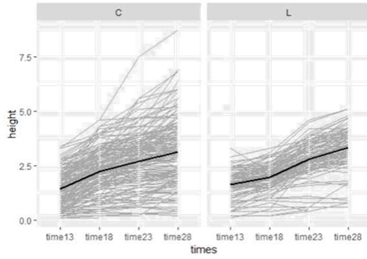
(b) Examine spaghetti plots of the plant heights across the measurements for each of the species (coneflower and leadplant). Is it reasonable to assume linear growth between Day 13 and Day 28? Does the initial height and/or rate of growth seem to differ between the species? Is there more variability in one species than the other?

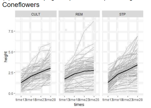
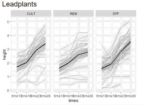
(c) Examine spaghetti plots of the plant heights over time separately for the three types of soil, separately for each species. What do you learn?

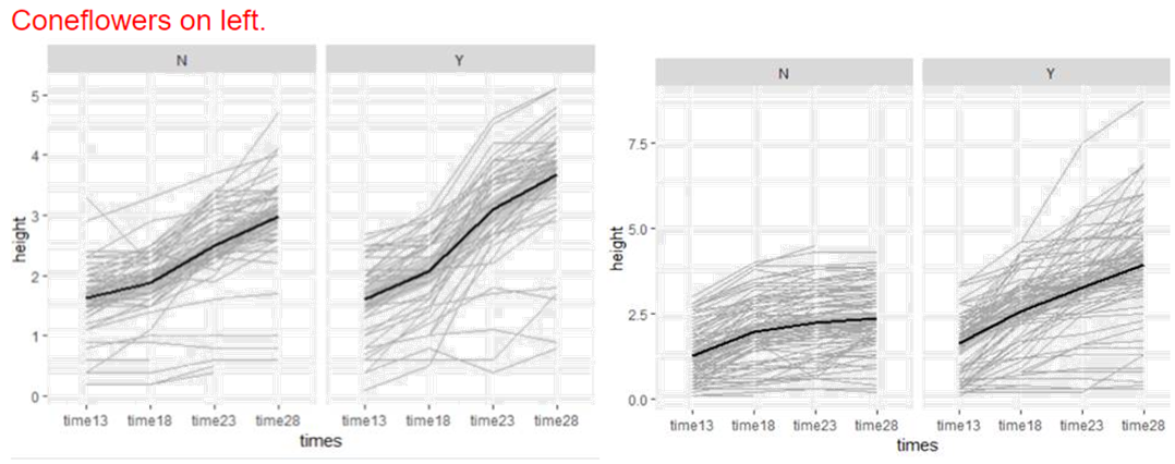
(d) Examine spaghetti plots of the plant heights over time separately for the two levels of sterilization, separately for each species. What do you learn?

Focusing on just the leadplants

(e) I next calculated time13 = time – time 13. Give two reasons this could be a good idea.

(f) Then I fit an “unconditional means” or “random intercepts” model with no predictors.

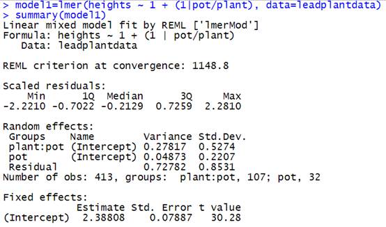
How many parameters are estimated? Provide an interpretation of each, including the variance components. Anything interesting about the relative size of the variance components?

(g) Next I included the new time variable in the model assuming linear growth.

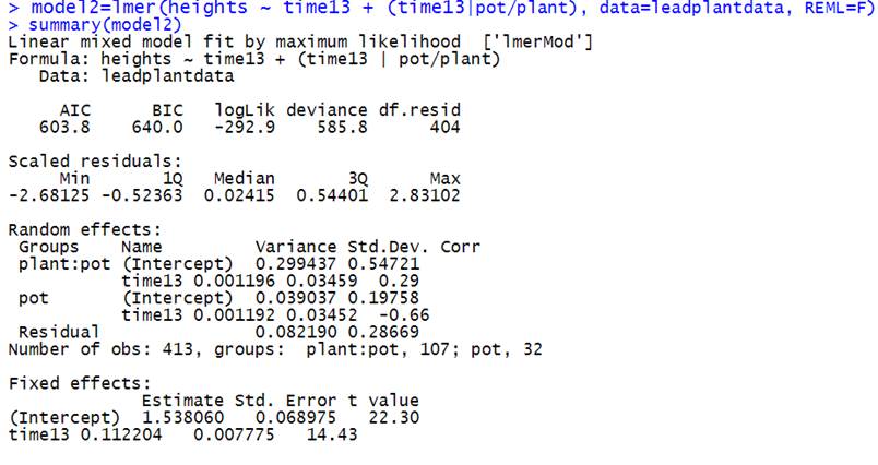
Explain what (time13|pot/plant) means to the model. Write out the theoretical level equations (in terms of ’s and being careful with indices). How many variance/covariance parameters are there/why?

How much of the within-plant variability is explained by the linear changes over time?

Interpret the fixed effects. Are either of the fixed effects statistically significant?

(h) Next I added the sterilization and soil type variables, including interactions with the time variable.

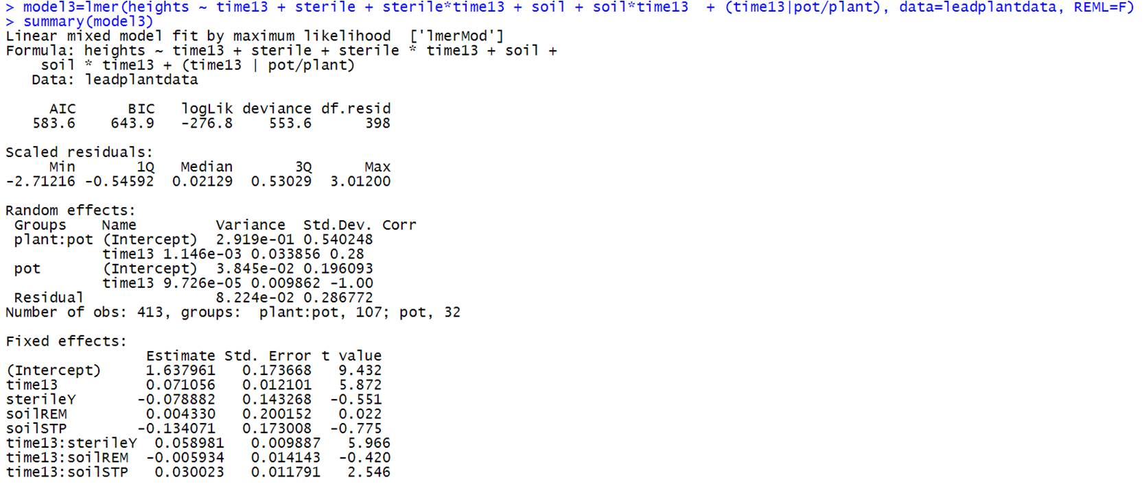
Why did I include interactions with the time variable? Is this model a significant improvement from the model in (g)?

(i) But this model in running into some boundary conditions. One option is to simplify the model, e.g., removing some variance/covariance components. Write out the model equations, for a new model so that the intercepts have random components at Levels 2 and 3 but the slopes are only allowed to vary at level 2. What is the practical interpretation of this modelling choice? How many parameters does this remove from the model?

[If you check, this model should be more stable, and not significantly worse.]

(j) Next we could consider adding an interaction between sterilization and soil type to the model, along with the three-way interaction between sterilization, soil type, and time.

How many parameters does this add? Interpret the nature of the three-way interactions. Explain what type of visual would help you assess the evidence of such an interaction.

(k) How would you change the previous model so that neither sterilization or soil type (or their interaction) are allowed to influence Day 13 measurements? Why might this be a reasonable consideration?

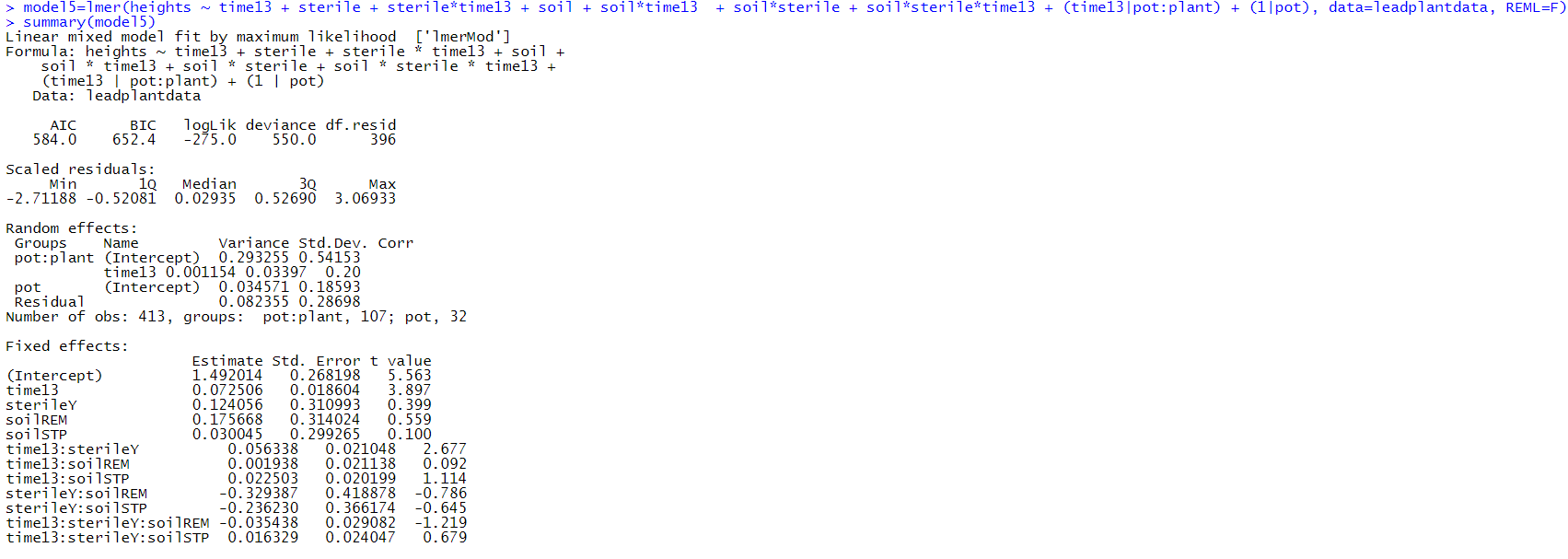
(l) Return to the fitted model in (i). Interpret it! (A brief summary of the important features, especially as the agree/disagree with your exploratory data analysis. What would the “effects plots” look like? What seems to maximize growth?!)