Stat 414 – Review 1 Problem Solutions

1) Data was collected on corn grown on the island of Antigua (corn.txt). The response variable is the harvest weight (harvwt) per plot (unknown units). There are eight sites with eight separate plots within each site where the corn is grown under the same treatment condition. One question of interest is whether site has an effect on harvest weight.

(a) Identify the response variable and the Level 1 units and Level 2 units.

Response variable = harvest weight

Level 1 units = plots

Level 2 units = sites

(b) Produce a graph of the harvest weights for the eight sites. Does there appear to be substantial site to site variation?

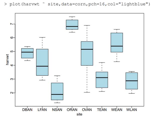
Yes, we do see substantial site to site variation, for example the ORAN site and NSAN site indicate very different havest weight values.

(c) Explain how we could use a traditional one-way ANOVA to model these data: identify the parameters, identify the error. Write out the statistical model (with proper indices, assumptions of error distribution, parameters).

Y_ij = harvest weight of ith plot in site j

Y_ij = + _j + e_ij j = 1, …, 8 sites, e_ij ~ N(0, ²)

where is the overall mean harvest weight in the population, _j is the fixed effect of the jth site, and ²is the within site variation (or the plot to plot variation, which we are assuming is the same for each site). For one-way ANOVA the _j are considered fixed effects; so these are the “effects” (not the group means, think effect coding).

(d) State null and alternative hypothesis and report a test statistic and p-value for assessing the site-to-site variation. Also produce a table of the estimated coefficients for the sites.

H₀: ₁ = …. = ₇ = 0

H_a: at least one _j ≠ 0

(So we only need 7 of them and we compare the set to zero, not just each other)

F = 17.4, df = 7 and 24, p-value < .0001. We have strong evidence that the population mean weights are these sites are not equal.

> summary(lm(harvwt~site, contrasts=list(site="contr.treatment"))) This gives indicator parameterization Coefficients: Estimate Std. Error t value Pr(>\|t\|) (Intercept) 4.8850 0.3800 12.856 2.96e-12 * siteLFAN -0.6775 0.5374 -1.261 0.219513 siteNSAN -2.7950 0.5374 -5.201 2.50e-05 * siteORAN 2.0300 0.5374 3.778 0.000922 * siteOVAN -0.0525 0.5374 -0.098 0.922984 siteTEAN -1.8487 0.5374 -3.440 0.002135 siteWEAN 0.6412 0.5374 1.193 0.244412 siteWLAN -2.0438 0.5374 -3.803 0.000865 ***	> summary(lm(harvwt~site, contrasts=list(site="contr.sum"))) This gives effect parameterization Coefficients: Estimate Std. Error t value Pr(>\|t\|) (Intercept) 4.29172 0.13434 31.946 < 2e-16 * site1 0.59328 0.35544 1.669 0.10808 site2 -0.08422 0.35544 -0.237 0.81471 site3 -2.20172 0.35544 -6.194 2.12e-06 * site4 2.62328 0.35544 7.380 1.28e-07 * site5 0.54078 0.35544 1.521 0.14121 site6 -1.25547 0.35544 -3.532 0.00170 site7 1.23453 0.35544 3.473 0.00197 **
By the way, there is a nice “display()” function in the arm package. But these are more about effects or group differences rather than estimates for the sites. > sapply(split(fitted(lm(harvwt~site)), site),mean) DBAN LFAN NSAN ORAN OVAN TEAN WEAN WLAN 4.88500 4.20750 2.09000 6.91500 4.83250 3.03625 5.52625 2.84125
So these do match the group means.

Now suppose we want to use a multilevel model. The main advantages are the ability to have plot level covariates, as well as site level covariates and an estimate of the error associated with the site level.

(e) Write out a statistical model for such a multilevel model, defining the parameters, with proper indices, assumptions of error distributions.

Y_ij = harvest weight of i^th plot in site j

Y_ij = + _j + e_ij j = 1, …, 8 sites, e_ij ~ N(0, ²) and _j ~ N(0, ²)

where is the overall mean harvest weight in the population, is the site to site variability, and ²is the within site variation (or the plot to plot variation, which we are assuming is the same for each site).

(f) State null and alternative hypothesis and report a test statistic and p-value for assessing the site-to-site variation.

H₀: = 0

H_a: > 0

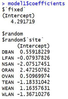
> model1=lme(fixed=harvwt~ 1, random = ~1 | site)

> model2=gls(harvwt~1)

> anova(model1, model2)

Model df AIC BIC logLik Test L.Ratio p-value

model1 1 3 100.4163 104.7183 -47.20816

model2 2 2 126.4154 129.2834 -61.20772 1 vs 2 27.99912 <.0001

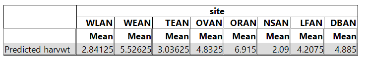
(g) Also produce a table of the estimated coefficients for the sites. How does these compare to the estimates from (d)? Why?

DBAN is first site, 4.291719 + .55918 = 4.851

> model1$fitted

fixed site

1 4.291719 4.850901

2 4.291719 4.212340

3 4.291719 2.216544

4 4.291719 6.764226

5 4.291719 4.801418

6 4.291719 3.108408

7 4.291719 5.455295

8 4.291719 2.924616

9 4.291719 4.850901

10 4.291719 4.212340

11 4.291719 2.216544

12 4.291719 6.764226

13 4.291719 4.801418

14 4.291719 3.108408

15 4.291719 5.455295

16 4.291719 2.924616

17 4.291719 4.850901

18 4.291719 4.212340

19 4.291719 2.216544

20 4.291719 6.764226

21 4.291719 4.801418

22 4.291719 3.108408

23 4.291719 5.455295

24 4.291719 2.924616

25 4.291719 4.850901

26 4.291719 4.212340

27 4.291719 2.216544

28 4.291719 6.764226

29 4.291719 4.801418

30 4.291719 3.108408

31 4.291719 5.455295

32 4.291719 2.924616

> sapply(split(fitted(model1), site),mean)

DBAN LFAN NSAN ORAN OVAN TEAN WEAN WLAN

4.850901 4.212340 2.216544 6.764226 4.801418 3.108408 5.455295 2.924616

DBAN decreased from 0.593 to 0.559. All of the estimated effects got closer to zero because of the “shrinkage” that occurs when we treat them as random effects. (So the estimated group means shrink towards 4.2819 – for example DBAN decreases from 4.885 to 4.851, WLAN increased from 2.841 to 2.925.

(h) Estimate and interpret the intraclass correlation coefficient. (How does this compare to R² from the one-way ANOVA?)

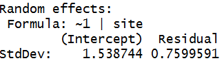
ICC = 2.3677/2.94527 = .8039, about 80% of the variation in response is at the site level. It’s a little lower because we are now assuming more variation in the data to be explained (MSTotal for the fixed model is 2.176).

This is in the ball park of R²

(i) Examine the residuals vs. fits graphs for this model and summarize what you learn.

plot(model1)

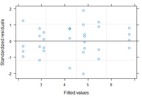
There does not appear to be huge violations in terms on linearity (though not really a condition in this one-way anova type model but don’t see any concerning patterns) or equal variance.

Below are the standard deviations of the residuals per level. We do have some that are more than twice the size of others (e.g., OVAN and DBAN).

2) A researcher is interested in seeing how different light conditions (Long = 16 hr days, Short = 8 hr days) affects the concentration of an enzyme in golden hamsters in heart tissue. Ten hamsters are randomly placed into each of the two light treatment groups, for a total of twenty hamsters. After a treatment period of several weeks, the hamsters are sacrificed and enzyme concentration (mg/ml) is measured in four subsamples of heart tissue for each hamster. The data is in the file hamster.txt. The primary research question is to compare the effects of light on the enzyme concentration in heart tissue.

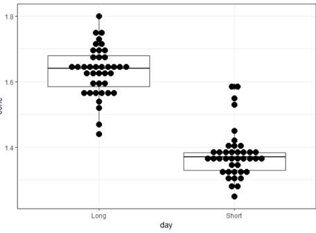
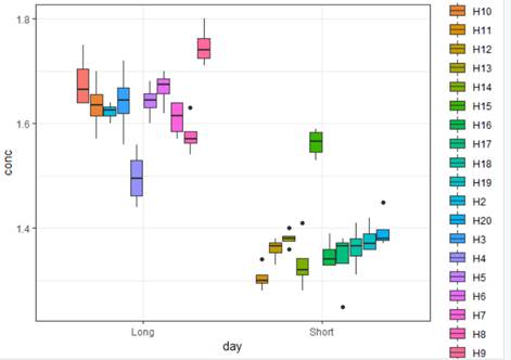
(a) Display a graph that highlights the primary research question.

Clearly the long day is associated with higher concentrations of the heart enzyme. There is variation in the measurements within each hamster, but that is smaller than the treatment to treatment variation. The within group variation in the hamsters looks pretty similar.

ggplot(hamsters, aes(y=conc, x = day, fill = id)) +

geom_boxplot()+

# geom_dotplot(binaxis='y', stackdir='center', dotsize=1) +

theme_bw()

(b) Fit and interpret a model that addresses the primary research question. Summarize your results.

Fitting a linear model between concentration and day with hamsters as a random effect (following a normal distribution). (Note: You could consider using a no intercept model here as there should not be any concentration on day 0.)

> model1= lmer(conc ~ day + (1 | id))

> summary(model1)

Linear mixed model fit by REML ['lmerMod']

Formula: conc ~ day + (1 | id)

REML criterion at convergence: -227.7

Scaled residuals:

Min 1Q Median 3Q Max

-2.30009 -0.54445 -0.03795 0.54010 1.93376

Random effects:

Groups Name Variance Std.Dev.

id (Intercept) 0.004216 0.06493

Residual 0.001644 0.04055

Number of obs: 80, groups: id, 20

Fixed effects:

Estimate Std. Error t value

(Intercept) 1.63225 0.02151 75.884

dayShort -0.25550 0.03042 -8.399

The t-statistic for dayShort is -0.255 / 0.0304 = -.12775/.01521 = -8.4, which is large (I consider anything larger than 2 in absolute value to be large), giving us convincing evidence that, after adjusting for the hamster to hamster variation, the mean concentration increases with time.

With indicator parameterization, the intercept predicts the mean concentration for the Long day treatment to be 1.63225 (with standard error 0.02151) or 1.37675 for the Short day treatment for the average hamster.

The dayShort slope estimates that the average concentration with the Short day treatment will be 0.2555 lower than average Long day treatment concentration for the average hamster.

An approximate 95% confidence interval for the difference (long minus short) is -.255 + 2(.030) or (0.195, 0.315).

This was a randomized experiment, so we can conclude that the Long treatment causes an increase in the concentration of the heart enzyme.

The hamsters explain .004216/(.004216 + .001644) or 71.9% of the random variation in the concentrations, after adjusting for the treatments.

(a) A has the largest ICC because the variation between the schools is the largest and B has the smallest ICC.

(b) The estimated effect would increase because there would be less shrinkage to the overall mean due to the larger sample size.

(a) 90.86

(b) 90.86 – sqrt(10.66)

(d) 90.86 + 3.113