Stat 414 – HW 2

Due midnight, Friday, Oct., 1

Please remember to upload each problem as a separate file. I’m giving you a lot more R help this time, so (a) please check it early in the week and (b) let us know about improvements! Also, feel free to use the book’s display function for nicer regression output?

install.packages("arm")

library(arm)

display(model1)

1) The data in child.iq.dta contains children’s cognitive test scores (“IQ”) at age 3, mother’s education, and the mother’s age at the time she gave birth for a sample of 400 children. I think the data also come from the National Longitudinal Survey of Youth as in Ch. 3.

library(haven) #need this package to read in a file in “Stata” format

child_iq <- read_dta("https://rossmanchance.com/stat414/data/child.iq.dta")

head(child_iq)

(a) Fit a simple linear regression model of child test score (ppvt) on mother’s age. Include a graph showing the scatterplot with the fitted model superimposed.

summary(model1 <- lm(ppvt ~momage, data=child_iq))

library(tidyverse)

ggplot(child_iq,aes(x=momage,y=ppvt))+geom_point()+

geom_line(aes(y=predict(model1))) +

theme_bw()

Interpret the slope coefficient in context. Based on this analysis, can we conclude that mothers should have children later to increase the intelligence of their children?

(b) Verify the t-statistic for mom’s age in the above output, including an interpretation, in context, of the standard error of the coefficient in this model. Is the t value above 2?

(c) The educ_cat variable here stands for mom's education where 1= no hs education, 2= hs grad, 3= some college, and 4= college grad. Now include mother’s education (as is) in the model.

summary(model2 <- lm(ppvt ~momage + educ_cat, data=child_iq))

Interpret both slope coefficients in this model. Have your “conclusions” about the timing of birth changed?

(d) Now include mother’s education as a factor.

summary(model3 <- lm(ppvt ~momage + factor(educ_cat), data=child_iq))

Which model (2 or 3) would you recommend? How are you deciding? (You should be clarifying the distinctions between the models and any assumptions behind them?)

(e) Now create an indicator variable reflecting whether the mother has completed high school or not. Include interactions between the high school completion variable and mother’s age. Also include a graph that shows the separate regression lines for each high school completion group.

child_iq$hs <- ifelse(child_iq$educ_cat >= 2, 1, 0) #one option, extra credit for others

summary(model4 <- lm(ppvt ~ momage*hs, data = child_iq))

ggplot(child_iq,aes(x=momage,y=ppvt,color= factor(hs)))+geom_point()+

geom_line(aes(y=predict(model4))) +

theme_bw()

Carefully and in detail interpret the interaction term in context. Should the interaction term be retained in the model? Justify your recommendation.

(e) Finally, fit a regression of child test scores on mother’s age and education level (high school or not) for the first 200 children and use this model to predict test scores for the next 200. Graphically compare the predicated and actual scores for the final 200 children.

summary(model5 <- lm(ppvt ~ momage*hs, data = child_iq[1:200, ]))

preds <- predict(model5, child_iq[201:400, ])

plot(preds ~ child_iq$ppvt[201:400], xlab="actual", ylab="predicted")

abline(a = 0, b=1)

sum((child_iq$ppvt[201:400] - preds)^2)

anova(model5)

How did we do? (Hint: What am I asking you to think about in the last 2 lines?)

2) Poisson regression

What do I do with count data, which is often skewed to the right and the variability increases with the mean?

Data on unprovoked shark attacks in Florida were collected from 1946-2011. The response variable is the number of unprovided shark attacks in the state each year, and potential predictors are the resident population of the state and the year.

(a) Create a graph of the number of attacks vs. year and vs. population. Do the graphs behave as expected? Does the conditional distributions appear skewed to the right? Does the variability in the response seem to increase with the number of attacks? Do the residuals show any issues with the linear model?

sharks <- read.table("https://rossmanchance.com/stat414/data/sharks.txt", header=TRUE)

head(sharks)

plot(sharks)

sharks$Year_coded <- factor(sharks$Year_coded, levels = c("45-55", "55-65", "65-75", "75-85", "85-95", "95-05", "05-15"))

ggplot(sharks, aes(x=Attacks)) + geom_histogram() + facet_wrap(~Year_coded)

model1 <- lm(Attacks ~ Year, data=sharks)

plot(model1)

Instead of assuming the conditional distribution are approximately normal, we can model them as Poisson distributions. The extension of the basic linear regression model is the general linear model. The Poisson regression model fits the model

where the observed y_i values are assumed to follow a Poisson distribution. The log transformation here is referred to as the “link function” and expresses how the response is linearly related to the explanatory variable. We’ve been doing a special case, the “identity” link and the normal distribution for the errors.

(b) Fit a Poisson regression model to these data.

model2 <- glm(Attacks ~ Year + Population, data=sharks, family=poisson)

summary(model2)

ggplot(sharks,aes(x=Year,y=Attacks))+geom_point()+

geom_line(aes(y=exp(predict(model2)))) +

theme_bw()

Interpret the coefficient of Year in this model, keeping in mind what you learned last week about (natural) log transformations.

There isn’t a perfect model and we won’t try to address everything here (e.g., modelling rates instead of counts), but we will consider the economic downturn after 9/11/2001, followed by a recession in 2008-2001, and very tropical weather in 2004, 2005, 2006. All of these contributed to fewer people going in the water, as well as increased awareness on the prudence of not provoking sharks.

(c) Fit the following model and summarize what you learn. I especially want to hear about the interaction here.

sharks$post911 = as.factor(sharks$Year >= 2002)

model3 <- glm(Attacks ~ Year*post911 , data=sharks, offset=log(Population), family=poisson)

summary(model3)

ggplot(sharks,aes(x=Year,y=Attacks))+geom_point()+

geom_line(aes(y=exp(predict(model3)))) +

theme_bw()

#or better yet

#library(ggeffects)

plot(ggeffect(model3))

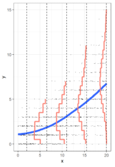
2) Weighted regression. Using the Squid data, let’s look at a couple simplified cases.

Squid<-read.table("http://www.rossmanchance.com/stat414/data/Squid.txt",header=TRUE)

model1 <- lm(Testisweight ~ DML, data = Squid)

SquidBel300 = as.numeric(Squid$DML < 300)

model2 <- lm(Testisweight ~ DML, data = Squid, weights = SquidBel300)

model3 <- lm(Testisweight ~ DML, data = Squid, weights = 1/DML)

plot(Testisweight ~ DML, data = Squid)

abline(model1); abline(model2, col="red"); abline(model3, col="blue")

(a) Explain what model 2 is doing. (Hint: How does it compare to lm(SquidBel300$Testisweight~ SquidBel300$DML))?

(b) Which model has the smallest slope? Why?

(c) How does the blue slope compare?

(d) The weighted regression that had the variance proportional to DML didn’t seem all that helpful. Let’s try a weighted regression that assumes the standard deviation is proportional to DML.

model4 <- lm(Testisweight ~ DML, data = Squid, weights = 1/DML^2)

plot(model4, which = c(1,2))

plot(rstandard(model4)~fitted.values(model4))

Is this an improvement? How are you deciding?