Kentucky Math Scores

Data were collected on 48,058 students from 235 middle schools from 132 different districts. These students were Kentucky eighth graders who took the California Basic Educational Skills Test in 2007. However, this analysis involves only 46,940 students who are complete cases. The variables of interests from this data set are:

- sch_id = School Identifier

- nonwhite = 1 if student is Not White and 0 if White

- mathn = California Test of Basic Skills Math Score

- sch_ses = School-Level Socio-Economic Status (Centered)

Main Objective

Is there a difference in math scores of eighth graders in Kentucky based on ethnicity and socioeconomic status, after accounting for the multilevel nature of the data.

(a) Summarize what you learn from the following graphs

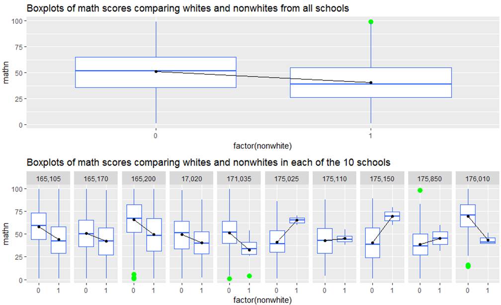
Overall, whites tend to have higher math scores than non whites, but we see there is quite a bit of variation in this comparison across schools. In some schools (e.g., 175205 and 175150, the nonwhites actually score quite a bit higher – though it also appears those are small sample sizes and may be a very selective group of test takers. Maybe there is some characteristic of those school that might explain this change in slope.

(b) Summarize what you learn from the following graph

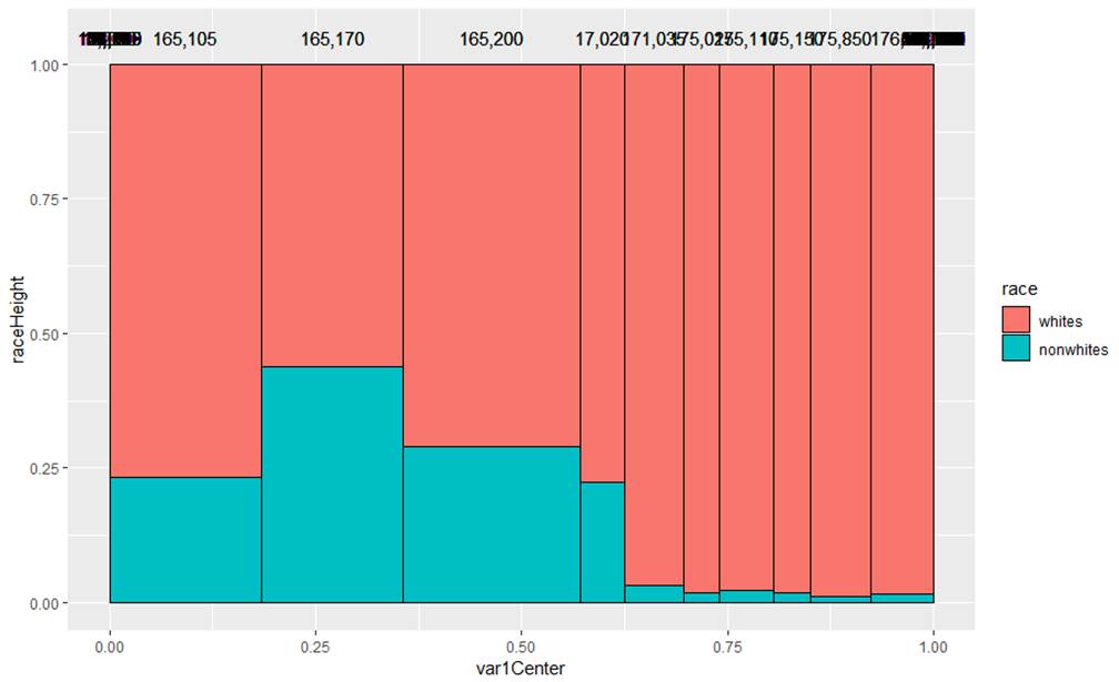
This is graph is not very well labeled, it’s actually the racial breakdown for 10 of the schools. The different width shows us the relative school size. We see that the smallest schools have very few nonwhites.

(c) Summarize what you learn from the following graphs

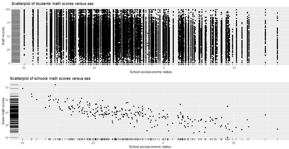
Overall there is a negative association between math score and the social economic status of the school though we see LOTS of within school variation in those math scores in the top graph. The bottom graph helps us see the overall trend but ignores that within school variability.

[It is kind of surprising to see that as ses increases, mean math scores tend to decrease. A possible explanation is that this test is only for students at the basic level, hence the name “California Basic Educational Skills Test.” So schools that are low ses have more basic level students taking it and they tend to do better. However, schools that are high ses have fewer basic level students taking it and they tend to do worse?]

(d) For each school separately, I have run a traditional regression to predict math score from student race (1 = nonwhite, 0 = white). For each school, I saved the intercept and slope of that regression. Below are the results

> summary(intercepts) Min. 1st Qu. Median Mean 3rd Qu. Max. 31.0 45.9 49.8 50.1 54.3 77.4 > summary(slopes) Min. 1st Qu. Median Mean 3rd Qu. Max. NA's -34.190 -14.986 -8.610 -6.799 0.061 34.955 21

Briefly summarize what you learn.

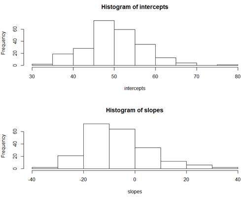
The intercepts represent the predicted math scores for nonwhite = 0, i.e., white students. We see that the predicted math scores for white students is about 50 pts on average across all schools. The slopes represent the difference in the predicted math scores from the whites to the nonwhites. We see that nonwhites are estimated to have a lower math score than whites by 7 pts on average across all schools. But we see lots and lots of variability in these slopes and intercepts across the schools. (If you look at the descriptive statistics – also where I got the means mentioned - SD for intercepts is about 7 pts and the SD for the slopes is about 12 pts)

These are the group means and standard deviations from the raw data. Notice this would have estimated about 12-13 points lower for the nonwhites on average.

> summary(math$mathn[math$nonwhite == 1])

Min. 1st Qu. Median Mean 3rd Qu. Max.

1.0 26.0 39.0 40.8 55.0 99.0

> summary(math$mathn[math$nonwhite == 0])

Min. 1st Qu. Median Mean 3rd Qu. Max.

1.0 36.0 52.0 51.1 65.0 99.0

(e) Summarize what you learn about the association between the slopes and intercepts.

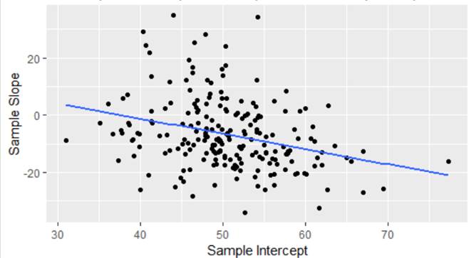
As sample intercepts increase, sample slopes tend to decrease. In context, as the predicted math score for white students increase, the difference between the whites and nonwhites becomes increasingly negative (larger difference between the whites and nonwhites). In schools where the white students score highly, there is more of a race gap than in schools where the whites don’t score as highly.

(f) Describe the nature of the association between ses and the sample intercepts and between ses and the sample slopes. Is there preliminary evidence that ses is a good predictor of the sample intercepts and sample slopes based on the associations? [Hint: What do these slopes represent?]

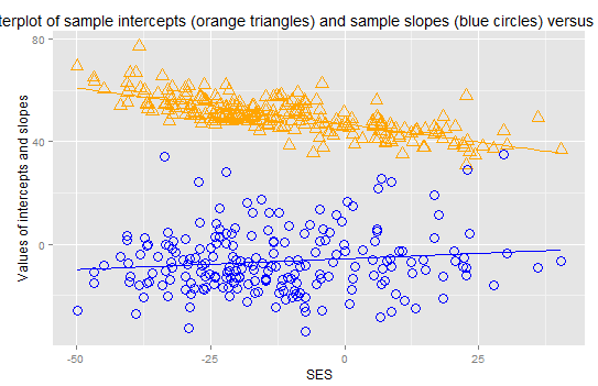
As school ses increases, the predicted math scores for white students decreases and the difference between whites and nonwhites gets less negative (closer to zero). Nonwhites tend to benefit from higher ses more than whites in regards to higher predicted math scores. Yes, there is preliminary evidence, stronger for intercepts than slopes.

(g) Below is output regression the intercepts on the school SES and the slopes on the school SES.

Summarize what you learn.

> model.intercept = lm(intercepts ~ mean.ses$x)

> summary(model.intercept)
 
Call:
lm(formula = intercepts ~ mean.ses$x)
 
Residuals:
 Min 1Q Median 3Q Max 
-13.112 -3.349 -0.659 2.549 19.742 
 
Coefficients:
 Estimate Std. Error t value Pr(>|t|) 
(Intercept) 46.8675 0.3616 129.6 <2e-16 ***
mean.ses$x -0.2811 0.0166 -16.9 <2e-16 ***
---
Signif. codes: 0 ‘***’ 0.001 ‘**’ 0.01 ‘*’ 0.05 ‘.’ 0.1 ‘ ’ 1
 
Residual standard error: 4.71 on 233 degrees of freedom
Multiple R-squared: 0.551, Adjusted R-squared: 0.549 
F-statistic: 286 on 1 and 233 DF, p-value: <2e-16

Every one increase in ses is associated with a .281 decrease in the predicted math scores for whites.

> model.slope = lm(slopes ~ mean.ses$x)

> summary(model.slope)

Call:

lm(formula = slopes ~ mean.ses$x)

Residuals:

Min 1Q Median 3Q Max

-27.86 -7.48 -1.97 7.55 42.78

Coefficients:

Estimate Std. Error t value Pr(>|t|)

(Intercept) -5.7084 1.0210 -5.59 0.000000069 ***

mean.ses$x 0.0847 0.0460 1.84 0.067 .

---

Signif. codes: 0 ‘***’ 0.001 ‘**’ 0.01 ‘*’ 0.05 ‘.’ 0.1 ‘ ’ 1

Residual standard error: 12.2 on 212 degrees of freedom

(21 observations deleted due to missingness)

Multiple R-squared: 0.0157, Adjusted R-squared: 0.0111

F-statistic: 3.39 on 1 and 212 DF, p-value: 0.0671

Every one increase in ses is associated with a decrease in the whites “advantage” over nonwhites by .08467 (what was a negative coefficient becomes less and less negative)

Is either association statistically significant? How much of the variation in intercepts and slopes is explained by the school SES?

The school SES is a highly significant predictor of average math scores for whites (explaining 55% of the variation in intercepts) and is borderline significant for the change in average math scores between nonwhites and whites (explaining 1.6% of the variation in slopes).

(h) How do the above results compare to the “unconditional means” (null, random intercepts only) model?

> lmer(mathn ~ 1 + (1 | sch_id), REML=TRUE, data=math)
Linear mixed model fit by REML ['lmerMod']
Formula: mathn ~ 1 + (1 | sch_id)
 Data: math
REML criterion at convergence: 416975
Random effects:
 Groups Name Std.Dev.
 sch_id (Intercept) 6.32 
 Residual 20.40 
Number of obs: 46940, groups: sch_id, 235
Fixed Effects:
(Intercept) 
 49 

Rather than running the two separate regressions, we have run one simple multilevel model with no predictors.

49 is the predicted mean math score for the average school.

-hat = 20.40, this is the variability in students’ math scores (from the mean) within a school

Note how similar the first two values are to the summary stats from the raw data

> summary(math$mathn)
 Min. 1st Qu. Median Mean 3rd Qu. Max. 
 1.0 34.0 50.0 49.8 64.0 99.0 
> sd(math$mathn)
[1] 21.46
 

= 6.32, this is the school to school variability in the mean math scores (compare this to the standard deviation of the intercepts found above)

 
> sd(intercepts)
[1] 7.0059

(i) Calculate and interpret the intraclass correlation coefficient.

6.32²/(6.32² + 20.40²) = .0875

So this is not that large, so this says there isn’t that much school to school variability relative to the variability in the scores within the same scool, that there is much more variability among the students within a school than there is between schools. Remember how much “cleaner” the graph of the means was compared to the graph of math score for individual students.

So if we go back to the first set of boxplots, we see that math scores ranges from 0 to 100, but the school means were all pretty much in the 40-60 range. Taking the school ID into account doesn’t explain much of the variability in the data.

(j) Below is the multilevel model version of the analysis.

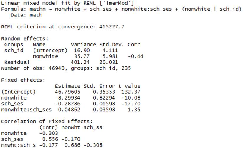
Interpret each estimated parameter.

= 46.8, this is our overall estimate the mean math score for whites.

= -8.3 this is the predicted change (decrease) in mean math scores for nonwhites compared to whites when school SES = 0 (the interaction)

= -0.283 this tells us the predicted change (decrease) in mean math scores with a one-unit increase in school SES for whites (nonwhite = 0)

= 0.0486 = this tells us about the difference in the effect of SES for whites and nonwhites. For whites, the overall effect of SES is negative (-.283). For nonwhites, the overall effect of SES is less negative (-2.83 + .0486). Similarly, as the SES increases, the difference between whites and nonwhites decreases (-.8299 + .0486 SES).

16.90 = this tells us about the school to school variation in mean math scores for whites after adjusting for SES (compare square root to the SD of the intercepts)

35.77 this tells us about the school to school variation in the race effect (difference in mean math scores for whites and nonwhites), after adjusting for SES (compare square root to SD of the slopes)

-0.44 = the correlation between the slopes and intercepts. The negative value shows that as the intercepts decrease (lower avg scores for whites) the slope coefficient increases (becomes less negative in this case as there is less of a distinction between whites and nonwhites).

Notice how much the variance in the intercepts has decreased by bringing in the school SES, now on par with the variation in the slopes.

We can also look at the random interceptslopess model with the race variable

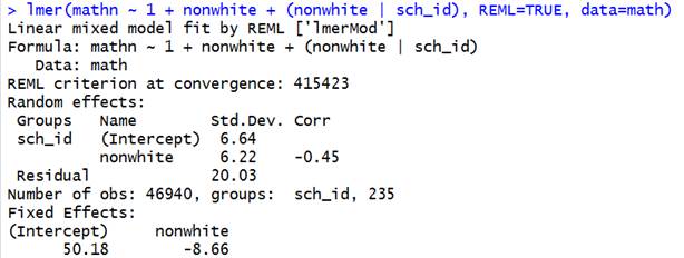
Adding SES explained some variation in the intercepts (school to school variation in avg scores for whites) (6.64 to 4.11) and some of the school-to-school variation in the effect of race (6.22 to 5.98)

(k) Which predictors would you consider significant?

The main effects of ses and race are significant but the interaction between the two is not (though more evidence here than in if we don’t account for the clustering in the data, see next question).

There is evidence that math scores differ by race and by ses separately, but the difference in math scores between race is not modified by ses (the regression of the slopes on SES was not a strong association, but the regression on the intercepts was).

(l) Below is a “one-level” analysis of the data, ignoring the school IDs.

> summary(lm(math$mathn ~ math$nonwhite + math$sch_ses + math$nonwhite:math$sch_ses))
 
Call:
lm(formula = math$mathn ~ math$nonwhite + math$sch_ses + math$nonwhite:math$sch_ses)
 
Residuals:
 Min 1Q Median 3Q Max 
-58.12 -14.48 0.39 14.14 65.96 
 
Coefficients:
 Estimate Std. Error t value Pr(>|t|) 
(Intercept) 46.39809 0.13353 347.48 <2e-16 ***
math$nonwhite -10.36714 0.40456 -25.63 <2e-16 ***
math$sch_ses  -0.30420 0.00562 -54.13 <2e-16 ***
math$nonwhite:math$sch_ses 0.00984 0.01771 0.56 0.58 
---
Signif. codes: 0 ‘***’ 0.001 ‘**’ 0.01 ‘*’ 0.05 ‘.’ 0.1 ‘ ’ 1
 
Residual standard error: 20.5 on 46936 degrees of freedom
Multiple R-squared: 0.0881, Adjusted R-squared: 0.088 
F-statistic: 1.51e+03 on 3 and 46936 DF, p-value: <2e-16

Do any of the conclusions change?

Now we would see very little evidence of an interaction, though other conclusions are similar.

(m) Why do you think our conclusion about the significance of the SES x race interaction is so different between these two approaches?

In the separate regressions exploration, we saw a bit more evidence of an interaction (significance of SES in the slopes, p-value = .067) and we see no evidence of an interaction in the one-level model (p-value = 0.58). The one-level model has not accounted for any school-to-school variation and this makes it more difficult to detect the subtle interaction. The separate regressions really doesn’t do any “pooling together” of information across the schools. The multilevel model is “between.” A small school with a large difference between whites and non-whites may be down-weighted a bit based on what is going on at the other schools.