Stat 301 – Review 2 Problems Solutions

1) Weights of 30 (fun-size) Mounds candy bars and 20 (fun-size) PayDay candy bars, in grams, are shown in the dotplots below.

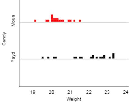
(a) Which distribution would you consider skewed to the right?

The Mounds distribution is a bit skewed to the right and the PayDay distribution is strongly skewed to the left.

(b) Which distribution do you expect has a larger mean?

The PayDay distribution is clearly centered around larger values than the Mounds distribution.

The PayDay values are more spread out/less consistent than the Mounds distribution.

In other words, the Mounds weights are more consistent, but occasionally a few weight more. The PayDay distribution is less predictable and often has weights that are much lower than typical, perhaps the difference of one or two peanuts?

(d) Which distribution would you suspect will have its mean larger than its median?

Mounds because it is skewed to the right

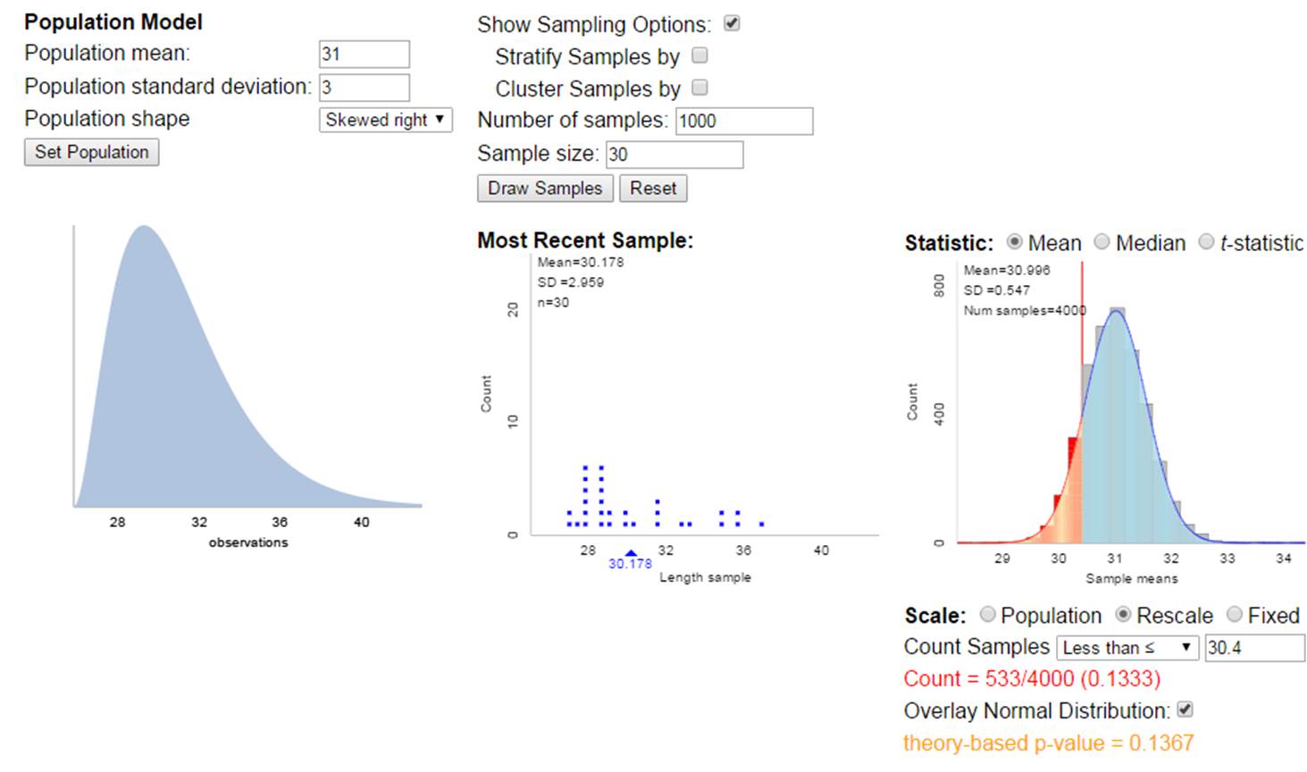
2) The highway miles per gallon rating of the 1999 Volkswagen Passat was 31 mpg (Consumer Reports, 1999). The fuel efficiency that a driver obtains on an individual tank of gasoline naturally varies from tankful to tankful. Suppose the mpg calculations per tank of gas have a mean of = 31 mpg and a standard deviation of = 3 mpg.

(a) Would it be surprising to obtain 30.4 mpg on one tank of gas? Explain.

Not really, 30.4 is well within one standard deviation of the “population” mean of 31.

z = (30.4 – 31)/3 = -0.20

(b) Would it be surprising for a sample of 30 tanks of gas to produce a sample mean of 30.4 mpg or less? Explain, referring to the CLT and to a sketch that you draw of the sampling distribution.

First, does the CLT apply here? We don’t know much about the shape of the population distribution, though it’s reasonable to assume the mileage from different tanks will by symmetric and roughly normal. But we also don’t care too much because our sample size of 30 is considered large. We are also assuming these observations are taken under identical conditions.

So we will model the distribution of the averages of 30 tanks for be normally distribution with mean equal to 31 and standard deviation equal to 3/sqrt(30) = 0.5477 mpg.

So a sample mean of 30.4 would be (30.4 – 31)/.5477 = -1.095 standard deviations below the mean. This is still not larger than 2.

Using the normal distribution, P(< 30.4)

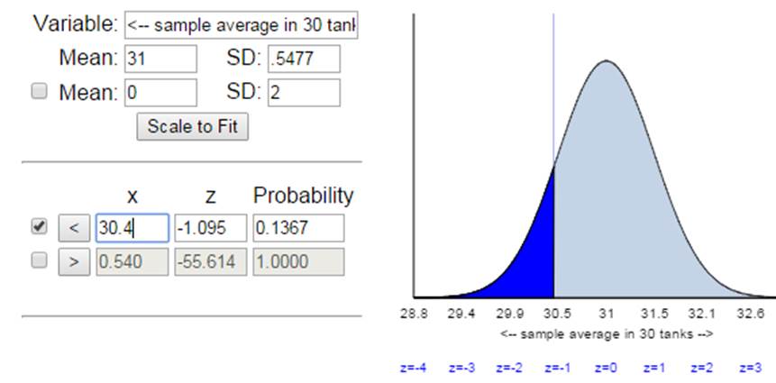
About 13.7% of samples of 30 tanks will have an average mileage of 30.4 by random chance alone. We would probably not consider this a surprising outcome.

It’s always reasonable to calculate a “standard score” as I did in (a). If I wanted to convert this z-value to a probability, then I would need to know that the tank MPGs follow a normal distribution. We aren’t told that here though it seems a reasonable assumption. As stated in (b), we can use the CLT if we continue to have this believe in the normality of the MPG values in general or if it’s reasonably close because then the sample of size 30 tells us that the distribution of sample means should still be approximately normal.

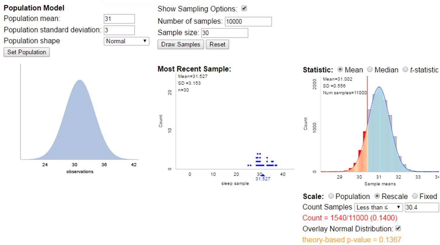
If you go to the Sampling from a Finite Population applet and check the box for Population Model, you can simulate drawing random samples from a probability distribution rather than a finite population. When the probability distribution is a normal distribution, everything works very well:

If the theoretical probability distribution is not normal but symmetric, things still work pretty well.

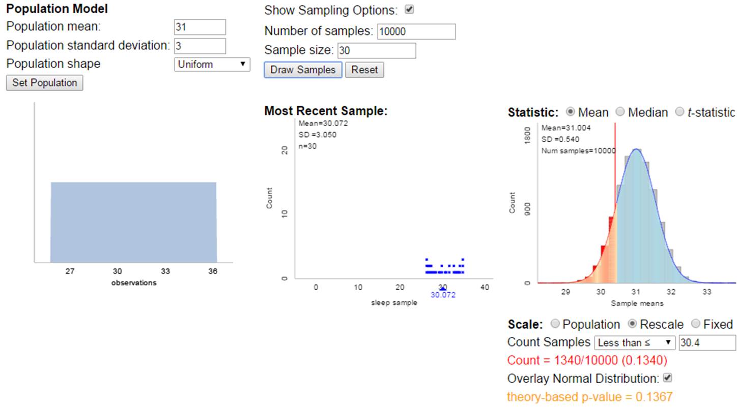
If the theoretical probability distribution is not normal to begin with, things still work pretty well due to the “large” sample size

3) The file AgeGuesses.txt contains students’ guesses of my age on the first day of class a few years ago.

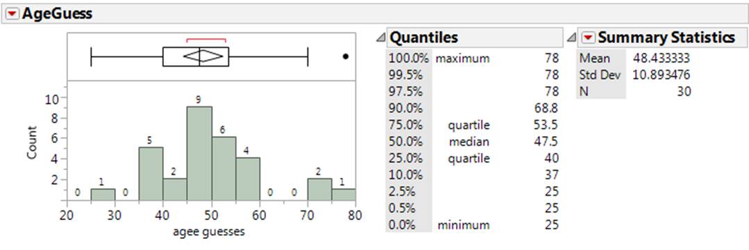
(a) Determine and interpret a 95% confidence interval for the population mean.

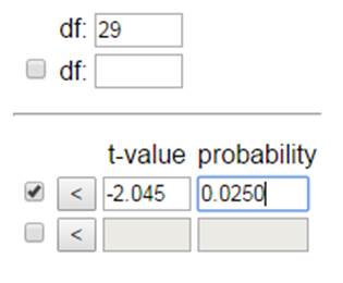
By hand: the t critical value for 95% confidence and 29 degrees of freedom is 2.045

+ t* (s /) = 48.43 + 2.045 (10.89/sqrt(30)) = (44.36, 52.50)

I’m 95% confident that the average guess of my age in the population of all Cal Poly students on such an activity would be between 44.36 and 52.50 years.

On an exam without the computer, for 95% confidence you can use 2 for either z* or t*.

(b) Determine and interpret a 95% confidence interval for the next student’s guess of my age.

+ t* (s ) = 48.43 + 2.045 (10.89 × sqrt(1+1/30)) = (25.79, 71.07)

I’m 95% confident that any one Cal Poly student would guess my age between 25.8 and 71.1 years.

Opinions will vary, the prediction interval is quite wide due to the huge amount of variation in the responses given to this question. Typically a prediction interval is more meaningful (what will happen next, vs. what is the long-run mean), but because it’s so wide this one is not very informative, basically saying I went to graduate school but I’m still alive!

(d) What information would you need to know to decide whether students’ are “biased” in how they guess my age in this activity? If you did a test of significance, would this be a one-sided or a two-sided test?

You would need to know my actual age, then we could see if the sample mean fell above that (overestimating my age on average) or below that (underestimating my age on average).

(e) Evaluate the validity of your calculations in (a) and (b).

The distribution is pretty symmetric and the sample size is 30 so the confidence interval in (a) is probably ok (achieves the stated 95% confidence in the long run) but with the outliers on both sides the distribution has heavier tails than we might expect for a normally distributed population. 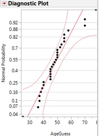If we believe these long tails exist in the population, then this would cast some doubt as to the validity of the prediction interval (though again, at least the distribution is symmetric, but there may be less than 95% of the population distribution falling within 2 standard deviations of the mean, or more if the population standard deviation is inflated by such outliers). The nonlinear nature of the normal probably plot suggests these data are not coming from a normally distributed population.

(f) Interpret the following JMP output

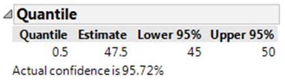
What is being estimated? What do you think is meant by “actual confidence” and why is it important?

This is a confidence interval for the median. I’m 95% confident that the median guess of my age by all Cal Poly students similar to those in this study would be between 45 and 50 years. The actual confidence is reporting how often we would expect the procedure used to actually capture the population median. We are pleased that this is close to the stated 95% confidence level.

(g) Column 2 indicates whether the data were collected in Section 1 or Section 2. I changed something about my appearance between the two sections. Suppose I find a statistically significant difference in the average guess of my age between the two classes, flipping a coin in advance to decide which appearance I would use in each section. Would you be willing to attribute the change in the ages to the change I made in my appearance? Explain why or why not.

While I did randomly assign the two treatments in a sense, I did so at the class level rather than at the individual student level. So there could still be a confounding variable between the two sections (e.g., I looked more tired later in the day) and we should not draw any cause-and-effect conclusion here. (Actually the average was 10 years larger in section 1!)

4) In a recent study (Klein, Thomas, and Sutter, 2007), researchers found that current smokers were more likely to have used candy cigarettes as children than current nonsmokers were.

(a) Identify and classify the explanatory and response variables.

EV = whether used candy cigarettes as child

RV = whether or not current smoker

(b) When first hearing of this study, someone responded by saying, “Isn’t the smoking status of the parents a confounding variable here?”

Explain what “confounding variable” means in this context, and describe how parents’ smoking status could be confounding (i.e., describe what would need to be true).

It would be a confounding variable if it provides an alternative explanation for the observed association. To do this, it must differ between the explanatory variable groups and potentially impact the response variable. So if those with smoking parents are more likely to be allowed to play with candy cigarettes as children but also more likely to smoke due to the environment they were raised and/or genetics, then the smoking habits of the parents might better predict who is a later smoker, but would also explain why current smokers are more likely to have played with candy cigarettes.

5) Newspaper headlines proclaimed that chocolate lovers live longer, following the publication of a study titled “Life is Sweet: Candy Consumption and Longevity” in the British Medical Journal (Lee and Paffenbarger, 1998). In 1988, researchers sent a health questionnaire to men who entered Harvard University as undergraduates between 1916 and 1950. The study included 7841 men, free of cardiovascular disease and cancer. From the questionnaire they determined whether the respondents consumed candy “almost never” (3312 men) or “sometimes or often” (4529 men), and then they tracked the participants to determine whether or not they had died by 1993.

(a) Identify the observational units.

men

(b) Identify the response variable.

Whether or not the person had died by 1993.

Whether the person was classified a candy consumer (sometimes or often) or not a candy consumer (almost never)

(d) Was this an experiment or an observational study? If an experiment, was it a randomized, comparative experiment? If observational, was if a case-control study? This was an observational study because the candy-consumption levels were not imposed on the men in the study, the men in the study chose for themselves. This is probably best classified as a cohort study because they were identified, their candy consumption determined, and then followed for 5 years to determine the outcome for the response variable. This means its legitimate for us to use this data to estimate the probability of still being alive.

(e) Researchers found that of respondents who admitted to consuming candy regularly, 267 had died by the end of 1993, compared to 247 of the non-consumers of candy. Set up the calculation for Fisher’s Exact Test for deciding whether candy consumers are significantly less likely to have died than non-consumers by completing the following:

Note: The conditional proportions of death are 267/4529 = .05895 and 247/3312 = .07458

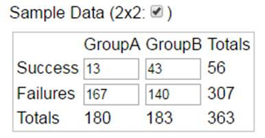
Best bet is to set up the two-way table:

	candy consumer	non-consumer	Total
still alive	4262	3065	7327
Died	267	247	514
Total	4529	3312	7841

If we let X represent the number still alive in the candy consumer group, then we want to find above X (even more survivors in candy consumer group)

p-value = P(X > 4262 ) where X follows a hypergeometric distribution with parameters

N = 7841 M = 7327 n = 4529

We can also look at the number deaths in the candy consumer group, which we expect (in the long run) to be less than the number of deaths in the non-consumer group. In this case, p-value = P(X < 267) where X follows a hypergeometric distribution with parameters N = 7841, M = 514, and n = 4529.

(There are other correct set ups as well.)

(f) The study reported: Between 1988 and 1993, 514 men died: 7.5% of non-consumers, but only 5.9% of consumers (age adjusted relative risk 0.83; 95% confidence interval 0.70 to 0.98). Interpret this statement as if to someone who has never taken a statistics class. In particular, what do you think is meant by “age adjusted relative risk”?

This interval provides an assessment for how much less likely a candy consumer is to die in this time frame than a non-consumer. The values in the interval are all less than one, so if we knew the death rate of non-consumers, we would multiply by .70 to .98 to find the death rate for those who eat candy.

“Age adjusted relative risk” essentially looks at the relative risks in different ages groups (so only comparing men of similar ages) and then roughly averages across those values to get an age-adjusted relative risk. This helps ensure we have “controlled” for age since we couldn’t do random assignment.

(g) Based on this interval, I would consider the comparison statistically significant. Why?

Yes, because 1 is not inside this 95% confidence interval, we know the two-sided p-value is less than .05.

(h) This does not appear to be a large difference (7.5% vs. 5.9%), are you surprised that this result is statistically significant? Explain.

1. No because the relative risk takes the magnitudes of the values into account. 1.6 percentage points may not be a lot but it’s a decent fraction of 5.9%.

2. The sample sizes are pretty large so even a weak association will probably end up being “statistically significant.”

~~(i) The study also reports:~~ We then examined different levels of candy intake. Compared with non-consumers, the relative risks of mortality among men who consumed candy 1-3 times a month (1704 men), 1-2 times a week (1589 men), and 3 or more times a week (1236 men) were 0.64 (0.48 to 0.86), 0.73 (0.55 to 0.96), and 0.84 (0.64 to 1.11),

~~Does this result provide evidence of a “dose-response”? Explain.~~

~~Yes, the relative “risk” of surviving that long is increasing with increasing amounts of candy!~~

(j) And then: Finally, using life table analysis truncated at age 95, we estimated that (after adjustment for age and cigarette smoking) candy consumers enjoyed, on average, 0.92 (0.04 to 1.80) added years of life, up to age 95, compared with non-consumers.

Based on these results, are you willing to conclude that eat candy leads to a longer life?

No, this was not a randomized comparative experiment, so we can’t draw any cause-and-effect conclusions.

A possible confounding variable is “happiness” – those who are happy and relaxed and not worried about what they eat are more likely to consume candy than those who are stressed and worried and watching their diet closely. But that happier lifestyle may also be responsible for longer lives.

(k) What population are you willing to generalize these results to? Explain.

At most well-off males (graduates from Harvard), but even that is risky as this study did not involve random sampling. It’s possible the access to medical care and long-life span for such individuals is not representative of all adults (certainly not women).

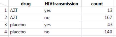
6) A study of whether AZT helps to reduce transmission of AIDS from mother to baby (Connor et al., 1994): Of the 180 babies whose mothers had been randomly assigned to receive AZT, 13 babies were HIV-infected, compared to 40 of the 183 babies in the placebo group.

(a) Create a segmented bar graph to display these results. Comment on what the graph reveals.

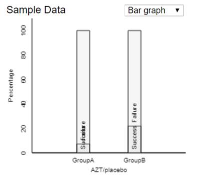
This bar graph (and the conditional proportions of 13/180 vs. 40/183) indicates that mothers given the placebo were about 3 times as more likely to have babies that were HIV positive than were the mothers given AZT.

(b) Check the validity conditions for whether a two-sample z-test can be applied to these data. Be sure to mention whether the study involves random sampling from populations or random assignment to treatment groups.

The number of successes and failures in each group should be at least 5. The four values are 13, 180-13 = 167, 40, 183-40=143. This condition is met.

(c) If you were to carry out a simulation to obtain a p-value, would you simulate random sampling or random assignment? Explain.

The data are from randomly assigning subjects to two treatment groups. So our p-value will want to reflect the random variation from random assignment (e.g., shuffling the 363 cards (53 successes and 310 failuers) to groups of 180 and 183).

(d) Conduct an appropriate test of significance to determine whether the data provide convincing evidence that AZT is more effective than a placebo for reducing mother-to-infant transmission of AIDS. Report the hypotheses, test statistic, and p-value. Also indicate the test decision using .01 as the level of significance.

The null hypothesis is that AZT and a placebo are equally effective in reducing mother-to-infant transmission of AIDS. Specifically, the probability of HIV-positive babies born to mothers who could potentially take AZT is the same as the probability of HIV-positive babies born to mothers who could potentially take a placebo. In symbols, the null hypothesis is H₀: π_AZT - π_placebo = 0.

The alternative hypothesis is that AZT is more effective than a placebo for reducing mother-to-infant transmission of AIDS, or that the probability of HIV-positive babies born to mothers who could potentially take AZT is smaller than the probability of HIV-positive babies born to mothers who could potentially take a placebo. In symbols, the alternative hypothesis is H_a: π_AZT - π_placebo < 0.

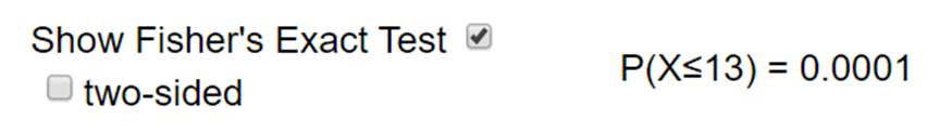
Because this is a randomized experiment and the counts are on the small size, we could carry out Fisher’s Exact Test.

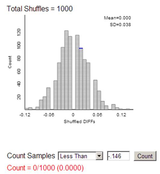
Or we could carry out the random assignment simulation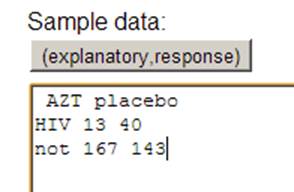

And find the p-value by counting how many re-random assignments have a difference in proportion with HIV positive babies (_AZT – _placebo) of -.146 or less

Or, because we said in (b) that the theory-based approach should be valid, we could go straight to the Theory-Based applet to carry out a ‘two-sample z-test’

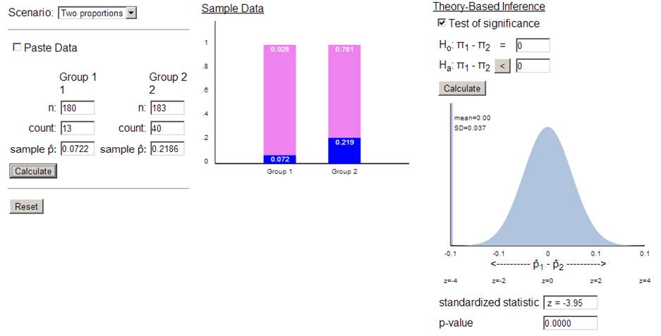
With such a small p-value, reject H₀ at the .01 level of significance.

We have very strong statistical evidence that AZT is more effective than a placebo for reducing mother-to-infant transmission of AIDS. We can say ‘more effective” because this was a randomized, comparative experiment.

(e) Estimate the difference in the risk of transmission is with AZT compared to a placebo with a 99% confidence interval. Also be sure to interpret this interval in context.

For a confidence level other than 95%, it is best to use the Theory-Based applet or JMP or R when the validity conditions are met. (Otherwise, we could take the SD from the null distribution but we would want a multiplier larger than 2 for 99% confidence, 2.576.)

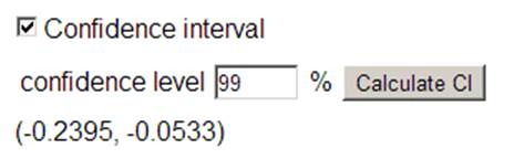
We are 99% confident the difference in HIV transmission rates is between 5.33 and 23.95 percentage points. As the values in our interval are all negative, we know that the AZT transmission rate is lower than the placebo transmission rate by somewhere between 5.33 to 23.95 percentage points.

Note: a confidence interval for the relative risk is probably more appropriate here. We could find one (95%) in the Two-way Table applet or JMP.

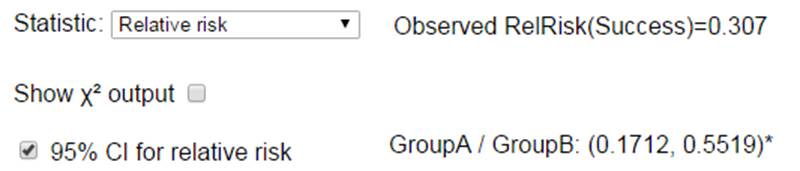
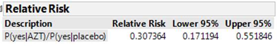
We are 95% confident that the risk of HIV transmission is 45% to 83% lower with AZT than with placebo.

If we set up the other way (larger than one):

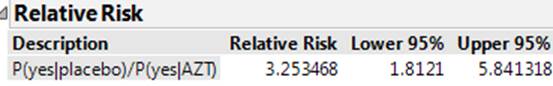
We are 95% confident that the risk of HIV transmission is 1.81 to 5.84 times larger with placebo than AZT.

(f) Summarize the conclusion that you could draw from this study (significance, estimation, causation, and generalizability). Also explain the reasoning behind each component.

Because this was a well-designed experiment with a small p-value, we can conclude that AZT caused the observed difference in HIV transmission rates. If AZT and a placebo were equally effective in reducing mother-to-infant transmission of AIDS, we virtually never see sample results as or more extreme as those we saw in this experiment by random assignment alone (p-value < .0001). We are 99% confident in concluding that AZT lowers the HIV transmission rate somewhere between 5.33 and 23.95 percentage points over that of a placebo, which seems noteworthy in this context. We might have some caution in generalizing these results to a larger population as we don’t know how the HIV-positive mothers willing to participate in this study were recruited.