Stat 301 – Review 2 Problems

1) Weights of 30 (fun-size) Mounds candy bars and 20 (fun-size) PayDay candy bars, in grams, are shown in the dotplots below.

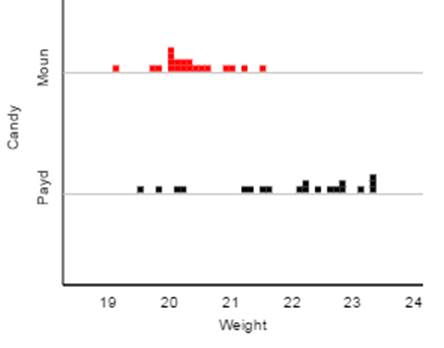
(a) Which distribution would you consider skewed to the right?

(b) Which distribution do you expect has a larger mean?

(c) Which distribution do you expect has a larger standard deviation?

(d) Which distribution would you suspect will have its mean larger than its median?

2) The highway miles per gallon rating of the 1999 Volkswagen Passat was 31 mpg (Consumer Reports, 1999). The fuel efficiency that a driver obtains on an individual tank of gasoline naturally varies from tankful to tankful. Suppose the mpg calculations per tank of gas have a mean of = 31 mpg and a standard deviation of = 3 mpg.

(a) Would it be surprising to obtain 30.4 mpg on one tank of gas? Explain.

(b) Would it be surprising for a sample of 30 tanks of gas to produce a sample mean of 30.4 mpg or less? Explain, referring to the CLT and to a sketch that you draw of the sampling distribution.

(c) Assess the validity of your calculations in (a) and (b).

3) The file AgeGuesses.txt contains students’ guesses of my age on the first day of class a few years ago.

(a) Determine and interpret a 95% confidence interval for the population mean.

(b) Determine and interpret a 95% confidence interval for the next student’s guess of my age.

(c) Which interval do you feel is more meaningful in this context?

(d) What information would you need to know to decide whether students’ are “biased” in how they guess my age in this activity? If you did a test of significance, would this be a one-sided or a two-sided test?

(e) Evaluate the validity of your calculations in (a) and (b).

(f) Interpret the following JMP output

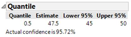
What is being estimated? What do you think is meant by “actual confidence” and why is it important?

(g) Column 2 indicates whether the data were collected in Section 1 or Section 2. I changed something about my appearance between the two sections. Suppose I find a statistically significant difference in the average guess of my age between the two classes, flipping a coin in advance to decide which appearance I would use in each section. Would you be willing to attribute the change in the ages to the change I made in my appearance? Explain why or why not.

4) In a recent study (Klein, Thomas, and Sutter, 2007), researchers found that current smokers were more likely to have used candy cigarettes as children than current nonsmokers were.

(a) Identify and classify the explanatory and response variables.

(b) When first hearing of this study, someone responded by saying, “Isn’t the smoking status of the parents a confounding variable here?” Explain what “confounding variable” means in this context, and describe how parents’ smoking status could be confounding (i.e., describe what would need to be true).

5) Newspaper headlines proclaimed that chocolate lovers live longer, following the publication of a study titled “Life is Sweet: Candy Consumption and Longevity” in the British Medical Journal (Lee and Paffenbarger, 1998). In 1988, researchers sent a health questionnaire to men who entered Harvard University as undergraduates between 1916 and 1950. The study included 7841 men, free of cardiovascular disease and cancer. From the questionnaire they determined whether the respondents consumed candy “almost never” (3312 men) or “sometimes or often” (4529 men), and then they tracked the participants to determine whether or not they had died by 1993.

(a) Identify the observational units.

(b) Identify the response variable.

(c) Identify the explanatory variable.

(d) Was this an experiment or an observational study? If an experiment, was it a randomized, comparative experiment? If observational, was it a case-control study?

(e) Researchers found that of respondents who admitted to consuming candy regularly, 267 had died by the end of 1993, compared to 247 of the non-consumers of candy. Set up the calculation for Fisher’s Exact Test for deciding whether candy consumers are significantly less likely to have died than non-consumers by completing the following:

p-value = P(X ) where X follows a distribution with parameters

N = M = n =

(f) The study reported: “Between 1988 and 1993, 514 men died: 7.5% of non-consumers, but only 5.9% of consumers (age adjusted relative risk 0.83; 95% confidence interval 0.70 to 0.98).” Interpret this statement as if to someone who has never taken a statistics class. In particular, what do you think is meant by “age adjusted relative risk”?

(g) Based on this interval, I would consider the comparison statistically significant. Why?

(h) This does not appear to be a large difference (7.5% vs. 5.9%), are you surprised that this result is statistically significant? Explain.

(i) The study also reports: We then examined different levels of candy intake. Compared with non-consumers, the relative risks of mortality among men who consumed candy 1-3 times a month (1704 men), 1-2 times a week (1589 men), and 3 or more times a week (1236 men) were 0.64 (0.48 to 0.86), 0.73 (0.55 to 0.96), and 0.84 (0.64 to 1.11),

Does this result provide evidence of a “dose-response”? Explain.

(j) And then: “Finally, using life table analysis truncated at age 95, we estimated that (after adjustment for age and cigarette smoking) candy consumers enjoyed, on average, 0.92 (0.04 to 1.80) added years of life, up to age 95, compared with non-consumers.“ Based on these results, are you willing to conclude that eat candy leads to a longer life?

(k) What population are you willing to generalize these results to? Explain.

6) A study of whether AZT helps to reduce transmission of AIDS from mother to baby (Connor et al., 1994): Of the 180 babies whose mothers had been randomly assigned to receive AZT, 13 babies were HIV-infected, compared to 40 of the 183 babies in the placebo group.

(a) Create a segmented bar graph to display these results. Comment on what the graph reveals.

(b) Check the validity conditions for whether a two-sample z-test can be applied to these data.

(c) If you were to carry out a simulation to obtain a p-value, would you simulate random sampling or random assignment? Explain.

(d) Conduct an appropriate test of significance to determine whether the data provide convincing evidence that AZT is more effective than a placebo for reducing mother-to-infant transmission of AIDS. Report the hypotheses, test statistic, and p-value. Also indicate the test decision using .01 as the level of significance.

(e) Estimate the difference in the risk of transmission with the placebo compared to AZT with a 99% confidence interval. Also be sure to interpret this interval in context.

(f) Summarize the conclusion that you could draw from this study (significance, estimation, causation, and generalizability). Also explain the reasoning behind each component.