Stat
301 - HW 6
Due
noon, Friday, Feb. 21
If you submit your assignment in Canvas,
remember to upload separate files for each problem and to put your name inside
each file. Remember to show your work/calculations/computer details and to integrate
this into the body of the solution.
1) In Wednesday’s lab, you used the Two
Population Proportions applet, but what if we wanted to explore another
statistic? Here are the R and JMP
equivalents for Example 1.
|
Push the green triangle to run the script. Right-click and choose Edit to see the script. You can change numsamples to 1000 and comment out the
“wait” lines. (Press Save or Done to update) On the mac, choose File > New Script and then copy the
contents of this file into that window. |
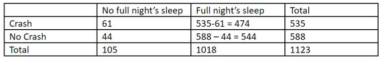
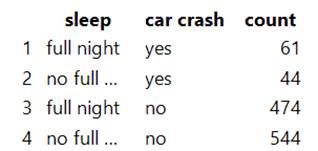
Because the Inv
3.11: sleep deprivation/car crash study is a case-control study (p. 232), we
should not use the data from that student to estimate the probability of a car
crash, either overall or in either group. Therefore, the difference in
proportions and relative risk are not recommended statistics. However, the odds ratio is a very relevant statistic.
Odds ratio = (number of successes group 1/
number of failures group 1) / ((number of successes group 1 / number of
failures group 2)) = ![]()
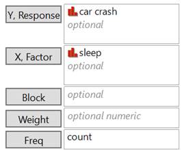
(a) Using R or JMP, modify the simulation from Wednesday’s
class to calculate the odds ratio each time.[Remember
to change the code in 2 places in JMP and in R to pick the correct code to
modify.] Include your histogram, summary statistics, and normal
probability plot. Is the mean of this
distribution close to what you expected?
Explain. (Make sure you include a copy of our code/script.)
Caution: I wouldn’t use the name “or” for your results.
[Alternatively, you can use the two-way table applet
to carry out the simulation, just keep in mind that it’s modelling random
assignment, not random sampling, and doesn’t provide normal probability plots.]
(b) Because the distribution is skewed to the right, a log
transformation might “normalize” the distribution. Take the natural log of the
odds ratios you generated in (a). Include output of a histogram, summary
statistics, and normal probability plot.
Would you consider this distribution to be approximately normal?
(c) Is the standard deviation of the distribution in (b)
similar to ![]() , where A, B, C, and D are the
four cell counts?
, where A, B, C, and D are the
four cell counts?
(d) Use the standard error from the formula in (c) to calculate
a 95% confidence interval for the population ln odds ratio. (You may still need to calculate the sample odds ratio for
this study)
(e) Back-transform the interval in (d) to estimate a 95%
confidence interval for the odds ratio.
Interpret your interval in context.
(f) Does the interval in (e) provide convincing evidence that
there is a significant association between whether or not New Zealand drivers
get at least one night sleep and whether or not they are involved in a car
crash the next week? Explain your
reasoning.
(g) Use JMP or R (or applet) to obtain a 95% confidence interval
for the odds ratio.
|
||||||||
|
|
2) When surveys are administered, it is hoped
that the respondents give accurate and honest answers. American researchers
investigated whether the mode of survey delivery affects respondents’
willingness to disclose socially undesirable information (Schober et al., 2015,
“Precision and Disclosure in Text and Voice Interviews on Smartphones”, PLOS One). They recruited people to
answer 32 questions from US social surveys via text messaging or speech,
administered either by a human interviewer or by an automated interviewing
system. In particular, question 6 asked
Voice:
“In a typical week, about how often do you exercise? ‘Less than 1 time per
week’, ‘1 or 2 times per week’, ‘3 times per week’, or ‘4 or more times per
week’?
Text:
“In a typical week, about how often do you exercise?
A. Less
than 1 time per week
B. 1 or
2 times per week
C. 3
times per week
D. 4 or
more times per week
We will focus how often respondents chose the “most extreme
categorical response option in the stigmatized direction” (less than 1 time per
week).
(a) Hypothesize a reason why someone might be less likely
to respond unfavorably to a human interviewer than to a text. Hypothesize a reason why someone might be
more likely to response unfavorably to a text than a human interviewer.
Suppose we had the following results
|
|
Text |
Call |
Total |
|
Success: Less than 1 time per week |
8 |
4 |
12 |
|
Failure: At least 1 time per week |
23 |
28 |
51 |
|
Total |
31 |
32 |
63 |
(b) Calculate the difference in conditional proportions,
the relative risk, and the odds ratio. Include
a one-sentence interpretation of each.
(c) State appropriate null and alternative hypotheses to
determine whether the delivery mode appears to influence how often individuals
choose the least desirable response.
(d) Use the hypergeometric distribution in JMP or R to
calculate a one-sided p-value, P(X > 8). (please
do one-sided) Show the details of your
calculation. (You can use technology, including the applet, to check your
answer for the p-value from Fisher’s Exact Test, but you should also demonstrate
that you can determine the p-value using the hypergeometric distribution
directly.)
(e) Is the two-sample z-test likely to be valid here? Calculate the pooled estimate of the standard deviation of ![]() 1 –
1 – ![]() 2 (p.189). Use the normal approximation to find the one-sided
p-value (e.g., Normal probability calculator applet) and then
verify the z-statistic and p-value
using R or JMP. How does
this p-value compare to the exact p-value?
2 (p.189). Use the normal approximation to find the one-sided
p-value (e.g., Normal probability calculator applet) and then
verify the z-statistic and p-value
using R or JMP. How does
this p-value compare to the exact p-value?
(f) One way to improve the normal approximation is to use a
continuity correction. Instead of
finding P(X > 8) = P(![]() 1 –
1 – ![]() 2 > 8/31 – 4/32),
we find P(X > 7.5) = P(
2 > 8/31 – 4/32),
we find P(X > 7.5) = P(![]() 1 –
1 – ![]() 2 > 7.5/31 – 4.5/32). Use the normal approximation (with the same standard
error as in (e)) to find this probability
2 > 7.5/31 – 4.5/32). Use the normal approximation (with the same standard
error as in (e)) to find this probability (and the
double it for a two-sided p-value). Is it closer to the exact
p-value?
3) Continue the previous study. The actual
data can be found here (PDTVISdata.csv)
and the codebook can be found here. Column B specifies the interview mode and
column D specifies whether or not they completed a required follow-up
debriefing. Column U contains the answer
to Question 6.
(a) Carry out the following data cleaning steps,
documenting your efforts:
·
Subset
the data file to only include those who completed the debriefing. (You should
now have 634 subjects.)
· Code the responses to the exercise
question to be “less than 1 time per week” or “at least one time per week”
|
R newQ6 = PDTVISdata$main_Q6 newQ6[newQ6 == 1] = "less
than once" newQ6[newQ6 == 2 | newQ6 == 3]
= "at least once" Also
search on “recode”? |
JMP Highlight the column you want to
recode. Select Cols > Recode. Change
the numbers so that you map some into the same category. |
·
Code
the interview modes to be text or call (see the codebook!)
Recreate a two-way table from the cleaned dataset.
(b) How do the statistics for the actual data compare to
what you found in problem 2(b)? How do you
expect the p-value for this data set to compare to what you found in problem 2(d)? Briefly explain.
(c) Carry out a two-sided,
two-sample z-test. Include the
output. How has the p-value changed, as you predicted?
(d) Use R, JMP, or applet
to calculate a 95% confidence interval for the relative risk of responding
“less than one time per week.” Include a one-sentence interpretation of the
interval, being especially clear on how you are defining the parameter and on
the direction of the difference you find.
|
R install.packages("fmsb")library(fmsb)riskratio(61, 44, 535, 588, conf.level=0.95, p.calc.by.independence=TRUE) |
JMP See the instructions in problem 1, and then use the hot
spot to select Relative Risk. Check
the box to calculate all combinations
and then pick one to interpret. |
(d) Does the confidence interval agree with the size of the
p-value? Explain how you are deciding.
(e) From the data file, use the original response and interview
mode results to create a 4x4 segmented bar graph (or mosaic plot). Summarize what you learn from the graph.
Possible Extension
Assignments
·
From
problem 3: If we want to compare the probability of responding “less than one
time per week” across the four categories, we could carry out 6 different
pairwise comparisons. What would be the problem with such “multiple testing” on
the same dataset?
·
Find
a study in the news that interprets a relative risk or odds ratio. Do they include a confidence interval? Do they include cautions about drawing cause
and effect conclusions? Do they “adjust” the estimate for other variables?
·
What
else did the researchers explore in the text vs. voice study?
·
From
problem 1: Do more investigation as to why the standard deviations for repeated
random sampling and re-random assignments differ. Can you explain why one is usually larger
than the other? Which one matches the theoretical formula better?
·
Participate
in SAFER survey and reflect on the experience