Stat 301 - HW 5

Due noon, Friday, Feb. 14©

If you submit your assignment in Canvas, remember to upload separate files for each problem and to put your name inside each file. Remember to show your work/calculations/computer details and to integrate this into the body of the solution.

R Users: You have the option of using the supplied RMarkdown file for problems 2 and 3. Click on the file and open it in RStudio (or copy and paste the contents into a New File > R Markdown. When you are done, press the Knit button. I prefer you knit to Word or PDF. If you knit to Word, you have the option of adding the discussion in Word rather than in the markdown file. Submit only knit Word or PDF files. You can run lines individual and preview the result. Remember that error messages apply to the entire chunk, not just the suggested line.

1) Complete the Stat 301 Midquarter Evaluation form in Canvas

2) Cohen et al. (2000) investigated whether the life expectancy of Major League Baseball umpires was less than expected. From an original list of 441 umpires, data were found for 227 who had died or had retired and were still living. Of these, dates of birth and death were available for 195 umpires. The data in Umpires.txt is the known lifetime (years) for the umpires who had died at the time of the study (censored = 0) and the current age of those who had not yet died (censored = 1). The “expected” column is the expected life length – from actuarial life tables –for individuals who were alive at the time the person first became an umpire.

(a) Load the data into JMP or R or use: hw5RMarkdown_2.Rmd. Subset the data to focus on those where we know how long they lived (i.e., censored ≠ 1).

In R:

load(url("http://www.rossmanchance.com/iscam3/ISCAM.RData"))

Umpdata = read.csv("http://www.rossmanchance.com/stat301/data/Umpires.txt", sep="", na.strings="*")

names(umpdata)

newumpdata = umpdata[umpdata$Censored != 1,]

nrow(newumpdata)

In JMP:

· Select Rows > Row Selection > Select Where

· Specify Censored = 1 and press OK

· Select Rows > Delete Rows (or just Hide/Exclude)

You should have 227 – 32 = 195 observations.

Create a new variable equal to the differences between how long each umpire lived and his expected life expectancy (actual – expected).

In R:

difference = newumpdata$Lifelength-newumpdata$Expected

hist(difference)

qqnorm(difference)

iscamsummary(difference)

In JMP:

· Select Cols > New Column

· Name the column Difference

· Use the Column Properties pull-down menu to select Formula

· Double click on no formula and enter

· Press OK twice and you should see the new column

Create (and include a screen capture of) a histogram and numerical summaries of this distribution of differences.

(b) Analyze the distribution (in context): Do the data appear to follow a normal distribution (e.g., examine/include a normal probability plot)? Does the shape of the distribution make sense in the context/what does it imply? What do the values of the mean and median imply (are they positive or negative) about this research question? Explain.

(c) Treating your differences as arising from a random sample of the umpire life expectancy process, define the parameter of interest, and state null and alternative hypotheses in terms of this parameter.

(d) Carry out a one-sample t test to decide whether baseball umpires (in general) tend to have smaller observed life lengths than expected (report the test statistic, p-value, degrees of freedom, and your conclusion in context). (You can also use the Theory Based Inference applet.) (Include your output.)

In R:

t.test(difference, mu = 0, alternative = "less")

In JMP:

· Choose Analyze > Distribution

· Specify the variable in the Y, Columns box

· Use the variable hot spot, select Test Mean. Then enter the hypothesized value of μ and press OK.

(e) Determine and interpret a 95% confidence interval for the parameter identified in (c). (Include your output.)

In R:

t.test(difference, mu = 0, conf.level = 0.95)

(R does assume a decimal confidence level)

In JMP:

· Choose Analyze > Distribution

· Specify the variable in the Y, Columns box

· The 95% confidence interval will be shown in the Summary Statistics box. If you want to change the confidence level, use the variable hot spot and select Confidence interval.

(f) Calculate a 95% prediction interval (show your methods). Provide a one-sentence interpretation of this interval in context.

(g) Discuss and evaluate the validity conditions for each of the t-procedures used in (d), (e), (f).

(h) What are the potential consequences of ignoring those 214 of the 441 umpires on the original list for whom data was unavailable?

(i) What are the potential consequences of ignoring those 32 umpires in the data set who had not yet died at the time of the study?

3) Measurements of e coli were taken in the San Luisito Creek (between here and Morro Bay) to assess the level of contamination from cattle grazing up river.

The data in SanLuisitoCreek.txt are from the “SLU” site near where the creek runs into Chorro Creek from Feb. 4, 2003 through Dec. 1, 2015.

R users: You are welcome to use this file: hw5RMarkdown_3.Rmd

(a) Produce (and include) a histogram of the E. Coli values, as well as a normal probability plot. Do these data appear to behave like a normal distribution?

(b) Take the (natural) log of the E. Coli values and create a normal probability plot of the ln e coli.

In R:

lnages = log(SanLuisitoCreek$E.Coli)

In JMP:

· Select Cols > New Column

· Name the column Difference

· Use the Column Properties pull-down menu to select Formula

· Double click on no formula and enter

(You can also try Transcendental > Ln and then double click on the column with the data…)

Do these data appear to behave more like a normal distribution?

(d) The measurement units of the interval in (c) is log-MPN/100ml, very difficult to interpret. We can back-transform the interval (LCL, UCL) by taking e (the base of our log transformation) to both endpoints: back-transformed interval = (e^LCL_,e^UCL). The one note is we will now interpret this interval to be for the population median rather than the population mean. Create and write a one-sentence interpretation of your interval.

(e) How does the confidence interval compare to the US EPA’s recommended full contact recreation limit for E. coli of 235 MPN/100 mL?

4) Researchers investigated whether owning a pet bird might be associated with having lung cancer. They studied a random sample of 239 lung cancer patients and an independent random sample of 429 people who did not have lung cancer, chosen to have similar characteristics to those with lung cancer. They asked all subjects whether they owned a pet bird in adulthood.

(a) Identify the explanatory and response variables in this study.

(b) Is this an observational study or an experiment? Justify your conclusion.

The researchers found that 98 of the lung cancer patients owned a pet bird, and 101 of those without lung cancer owned a pet bird.

(c) Why is it not appropriate to conclude that there is no association between whether or not you own a bird and whether or not you get lung cancer because 98 » 101?

(d) Organize these data into a 2×2 table, with the explanatory variable in columns.

(e) Calculate the proportion of subjects in this study with lung cancer. Is this an appropriate estimate of the probability of lung cancer in this population? Explain why or why not based on how the data were collected. (Hint: See Investigation 3.11)

(f) Create (and include) a segmented bar graph (p. 184) and summarize what it reveals about the association between bird ownership and lung cancer.

(g) State appropriate null and alternative hypotheses for testing whether the probability of lung cancer is larger for the bird owning population than the non-bird owning population.

(h) Using normal-based methods (as you should see Thursday), I found the following output

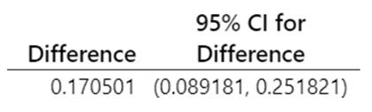
Summarize your conclusions from this analysis:

· Is the result statistically significant? How are you deciding?

· What is the estimated difference in the probability of lung cancer between the two populations? (in context)

· To what population are you willing to generalize these results? Justify your answer.

· Are you willing to conclude that owning a bird causes lung cancer? Explain why or why not. If not suggest a possible confounding variable.

Possible Extension Assignments

· For problem 3, explain the units of MPN/100ml

· For problem 3, explain why the confidence interval in (d) is about the median rather than the mean (See Investigation 2.8, cite any additional references.)

· For problem 3, suggest a question you might want to know about these data and the impact of cattle grazing that the above analysis does not address.

· For problem 4, create a mosaic plot rather than a segmented bar graph. (You can use the Analyzing Two-way Tables applet) How do the graphs compare/why? Which do you prefer?

· Find a scientific study that uses a method from Section 2.3 (e.g., bootstrapping, sign test, median rather than mean, transformation). Summarize what the article/study is about and what you did/did not understand about the analysis.