Stat 301 – Final Exam Review Solutions
1. Recall from
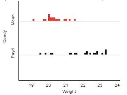
the exam 2 review problems the weights of 30 (fun-size) Mounds candy bars and 20 (fun-size) PayDay candy bars, in grams.
d) State null
and alternative hypothesis for comparing the means of these two distributions,
both in symbols and in words.
Let ![]() Mounds represent the long-run
mean weight for the Mounds manufacturing process and
Mounds represent the long-run
mean weight for the Mounds manufacturing process and ![]() PayDay the long-run meant weight for
the PayDay manufacturing process. We
want to know whether the observed difference in these sample means convinces us
that there is a genuine differences in the long-run mean weights for these two
manufacturing processes.
PayDay the long-run meant weight for
the PayDay manufacturing process. We
want to know whether the observed difference in these sample means convinces us
that there is a genuine differences in the long-run mean weights for these two
manufacturing processes.
H0: ![]() Mounds -
Mounds - ![]() PayDay = 0 (no difference in the
long-run means)
PayDay = 0 (no difference in the
long-run means)
Ha: ![]() Mounds -
Mounds - ![]() PayDay ≠ 0 (this is
a difference in the long-run means)
PayDay ≠ 0 (this is
a difference in the long-run means)
We
were just asked to compare the means, there was no prior suspicion given as to
which candy bars would be heavier, so we are using a two-sided alternative.
e) Do you think
a theory-based analysis would be appropriate for these data? Explain how you
are deciding.
It’s a little questionable, the sample sizes are
both at least 20 but we do have some skewness in the sample distributions (and
in opposite directions). Would probably be worth looking at a second
analysis as well.
d) Is this
distribution approximately normal? Would you have expected this? Explain
This distribution looks a bit skewed left,
consistent with our skepticism in question (c).
e) Would you
expect this distribution to follow a t distribution? Explain
Actually, the t model is for the
standardized statistics, not the distribution of the differences in sample
means. We don’t quite see the heaviness in the tails (because we aren’t using
the s’s yet) that we might for
the t distribution.
f) Use the
above output to roughly approximate the p-value. Explain how.
First
we have to roughly approximate the difference in sample means from the
original dotplots, keeping in mind that
the PayDay mean might be pulled a little
bit to the left of the main peak. Maybe 22.2 grams and 20.5
grams?? So say we think the difference in means is around 2
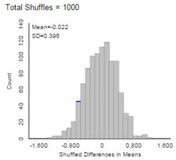
grams. Then we need to look at the randomization distribution and
see how often we get a difference of -2 or smaller or a difference of 2 or
larger for a two-sided p-value. However, we see 2 is off the chart
on both ends so this would approximate a p-value of zero. In reality the difference in
means is 1.605 grams, which is still pretty extreme and the empirical p-value
is zero.
g) Explain a
difficulty with using this simulation approach to analyze these data.
This is a randomization distribution, assuming
random shuffling of the weights to the two brands. But that is not
how the data were collected, that was through independent random sampling from
each random process. So we might prefer a simulation that reflecting
the randomness from sampling from an infinite process rather than from random
assignment (e.g., bootstrapping).
h) Assuming
it’s valid, how would you interpret this confidence interval?
![]()
I’m 95% confident that the mean weight of
(all) PayDay candy bars is .99 to 2.2 gram
larger than the mean weight of (all) Mounds candy bars.
2) A study
examined whether a nicotine lozenge can help a smoker to quit. The research
reports on many background variables, such as age, weight, gender, number of
cigarettes smoked, and whether the person made
a previous attempt to quit smoking (Shiffman et
al., 2002). Suppose the researchers want to compare the distributions of the
background variables between the two treatment groups (nicotine lozenge or
placebo lozenge).
(a) For each of the five variables listed,
indicate whether it calls for a comparison of means or a comparison of
proportions.
Age –
quantitative – means
Weight
– quantitative – means
Gender
– categorical – proportions
Number
of cigs smoked – quantitative - means
Previous
attempt – categorical – proportions
(b) Would the researchers hope to reject the
null hypotheses or fail to reject the null hypotheses in these tests? Explain.
In this case, large p-values would be good news –
it would provide more evidence that our treatment groups were similar to each
other at the beginning of the study so any differences observed at the end of
the study are even more safely attributed to the nicotine lozenge’s superior
effectiveness to the placebo lozenge.
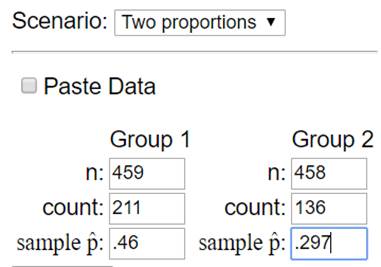
(c) Of the 459 nicotine users, 46.0% successfully abstained (didn’t
start smoking again) for 6 weeks, compared to 29.7% of the 458 control group
(without nicotine). Calculate and interpret a 95% confidence interval.
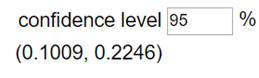
I’m
95% confident that the probability of abstaining is .1009 to .2246 larger when
assigned to nicotine rather than to the placebo.
(d)
Are you willing to draw a cause-and-effect conclusion from this study? If not,
suggest a possible confounding variable and explain how it is confounding in
this study.
Yes,
because there was random assignment to the treatment groups (nicotine or not)
(e)
Are you willing to generalize these results to all smokers interested in
quitting? If not, suggest a possible source of sampling bias and the likely
direction of the bias.
Maybe
not, we don’t have a lot of information about these individuals were
recruited. Maybe those willing to
participate in a smoking cessation study are different (more likely to abstain)
than those who want to quite but aren’t willing to participate in a research
study.
3) Researchers examined the long-term survival
of doctors graduating from one medical school over one
century (Redelmeier and Kwong,
2004), comparing those who were presidents of their class to those who appeared
alphabetically before or alphabetically after the president in the graduating
class photograph. Statistics on long-term mortality were obtained
from licensing authorities, medical obituaries, professional associations,
alumni records, and national physician directories (follow-up
94%). They reported on 507 presidents and 1014 classmates.
(a) Is it reasonable to
treat the presidents and non-presidents as independent random samples?
This is
a bit debatable, because they took all three from the same year, rather than
taking a random sample of presidents and then a separate random sample of non presidents. But
if we don’t think the variable changes too much from year to year, we could
treat them as independent samples. It might be better to more directly compare
the 3 classmates from each graduating class, but it’s not obvious how to do
that either. It’s not clear how the 507 were selected or is that all of the
presidents. This is also from just one
school.
Assuming the answer to (a)
is yes:
(b) The researchers examined
several base-line variables, including gender and whether or not the individual
wore glasses. They found 93% of the presidents were male, compared
to 85% of their classmates. They also found 9% of presidents were
glasses, compare to 12% of their classmates. Are either of these
differences statistically significant?
Because the response variables
here (sex and whether wore glasses) are categorical, we will consider the two-sample
z procedure. In both cases, we can define ![]() pres
pres ![]() classmate as the parameter of interest and then test hypotheses H0:
classmate as the parameter of interest and then test hypotheses H0: ![]() pres-
pres-![]() classmate = 0 (no difference in the population proportions) vs. Ha:
classmate = 0 (no difference in the population proportions) vs. Ha: ![]() pres-
pres-![]() classmate ≠ 0 (there is a difference in the population
proportions). Because the sample sizes are large, the two-sample z-procedures
are appropriate.
classmate ≠ 0 (there is a difference in the population
proportions). Because the sample sizes are large, the two-sample z-procedures
are appropriate.
JMP output for male/female comparison:
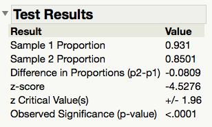
There is a statistically
significant difference (p-value <.001 < .05) in the sample proportion of
presidents who were male compared to the sample proportion of classmates who
were male. We are 95% confident that the population proportion of classmates
who are male is .05 to .11 lower than the population proportion of presidents
who are male.
Applet and JMP output for
glasses comparison:
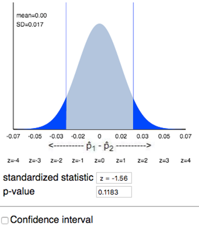
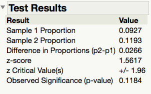
There is not a statistically
significant difference (p-value = .1187 > 0.05) in the proportion wearing glasses.
(c) The overall-life
expectancy for the presidents was 49.0 years compared to 51.4 years for their
classmates. The two-sided p-value was reported to be
.036. Assuming the sample standard deviations were similar in the
two samples, use trial-and-error in JMP or TOS applet or algebra to approximate
the value of this standard deviation. What conclusion would you draw
from this p-value?
Let ![]() pres represent the life-expectancy (mean lifetime) for all class
presidents and
pres represent the life-expectancy (mean lifetime) for all class
presidents and ![]() class represent the life-expectancy for all classmates.
class represent the life-expectancy for all classmates.
H0: ![]() pres - mclass
= 0 (no difference in the average life-expectancy between these two
populations)
pres - mclass
= 0 (no difference in the average life-expectancy between these two
populations)
Ha: ![]() pres ≠
pres ≠ ![]() class (there is a difference)
class (there is a difference)
If we use the conservative df of 506, a two-sided p-value of
.036 corresponds to t0 = -2.102.
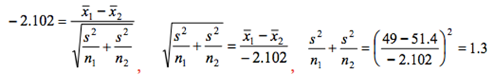
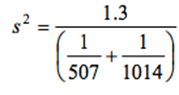 =439.4, so s = 20.96.
The sample standard deviation must have been close
to 21 years.
Using this value below to verify the p-value:
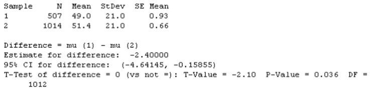
The
p-value of .036 provides moderate evidence (.01 < p-value < .05) of a
difference between the population mean life expectancy of the class presidents
compared to their classmates. We would reject the null hypothesis at the 5%
level.
4. Because
these were two different questions on the same survey, we shouldn’t apply a
“two-sample” procedure, but should treat the observations as paired instead.
5) In a study reported in the July 6, 2007 issue
of the journal Science, researchers studied 396 American college
students and kept track of each student’s sex and also how many words they
spoke in a day. They found that females spoke an average of 16,215 words per
day and males an average of 15,669 words per day.
Consider
the following variables:
- Sex
- Average number of words spoken per
day
- Number of adjectives used per day
- Proportion of words
spoken in a day by each student that were adjectives
- Whether more than 15,000 words were spoken
For each
research question below, which theory-based method would you consider:
·
One-proportion z-test or
interval
·
One-mean t-test or
interval
·
Two-proportion z-test or
interval
·
Two-mean t-test or
interval
Briefly justify your answer.
(a) Do women tend to use more words than men?
Two-mean t-test
(b)
How often does the proportion of adjectives a person uses in a day exceed 0.25?
In other words, estimate the probability more than 25% of the words someone
uses in a day are adjectives.
Confidence interval for one proportion (variable: whether or not
exceed .25; parameter: probability of exceeded 0.25.)
(c) Are women more likely than men to use more than 15,000 words
per day?
Two-proportion z-test
(d) Do people tend to talk more (use more words) on the weekends
or on the weekdays?
Paired t-test (difference in number of words) or one proportion
(probability of using more on weekend than weekday). The point is get one measurement per person
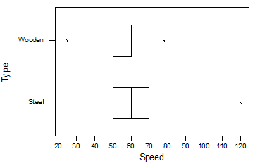
6)The Roller Coaster Database
maintains a web site (www.rcdb.com) with
data on roller coasters around the world. Some of the data recorded
include whether the coaster is made of wood or steel and the maximum speed
achieved by the coaster, in miles per hour. The boxplots display the
distributions of speed by type of coaster for 145 coasters in the United
States as of Nov. 2003.
(a)
Do these boxplots allow you to determine whether there are more wooden or steel
roller coasters?
No,
no sample size information presented
(b)
Do these boxplots allow you to say which type has a higher percentage of
coasters that go faster than 60mph? Explain and, if so, answer the
question.
50%
of steel go faster than 60 mph compared to 25% of wooden
(c)
Do these boxplots allow you to say which type has a higher percentage of
coasters that go faster than 50mph? Explain and, if so, answer the
question.
Both
types have 75% exceeding 50 mph.
(d)
Do these boxplots allow you to say which type has a higher percentage of
coasters that go faster than 48mph? Explain and, if so, answer the
question.
No,
because 48 mph does not match up with a quartile, we can’t say anything about
how the values compare to 48mph. We know nothing about how the lowest 25% are
distributed along those “whiskers.” In
particular, having longer whiskers doesn’t imply a higher percentage in that
area.
(e)
The steel coasters have a “high outlier.” Explain how I know this from the
above display and interpret this outlier in context. What would be your next
step in analyzing these data?
The
star plotted off on its own. This is a
coaster than goes much faster than all the rest. We should figure out which coaster it is. We
can also see how the distribution changes if that observation is removed.
(f)
Conjecture as to how the mean, median, interquartile range, and standard
deviation will change (if at all) if that coaster identified in part (e) (Top Thrill Dragster in Cedar Point Amusement Park,
Sandusky, Ohio) is removed from the data set. Explain your
reasoning.
Removing
a high outlier will lower the mean and even the median, but probably more
noticeably for the mean.
Removing
a high outlier that is far from the mean will lower the variability in the data
so the interquartile range and standard deviation will decrease, but probably
more noticeably for the standard deviation.