INVESTIGATING STATISTICAL CONCEPTS, APPLICATIONS, AND METHODS

BRIEF SOLUTIONS TO INVESTIGATIONS

Last Updated Nov. 26

Investigation 1-1: Popcorn Production and Lung Disease

(a) 21/116 = .81

(b) proportion in each group

(c)

	Low exposure	High exposure	Total
Airway obstructed	6	15	21
Airway not obstructed	52	43	96
Total	58	58	116

(e) There appears to be a higher rate of airway obstruction in the “high exposure” group.

(f) Low exposure: 6/58 =.103; High exposure: 15/58 = .259

(g) .259-.103 = .156, seems reasonably large

(h) .650-.494 = .156, same difference but doesn’t “feel” as large?

(i) .259/.103 = 2.51

(j) 21/95 = .22

(k) (15/43)/(6/52) = 3.02

Investigation 1-2: Smoking and Lung Cancer

(a) males

(b) EV = amount of smoking (categorical); RV = whether have lung cancer (categorical)

(c)

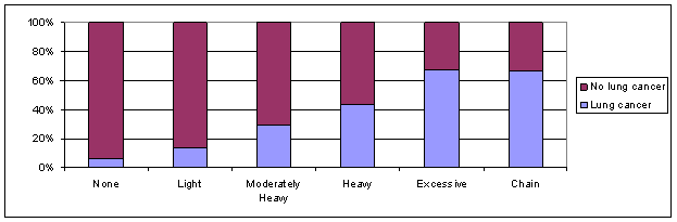
(d) 14/90 = .156; 8/114 = .070; ratio = 2.217

(e) (14´114)/(8´90)

(f) (213´114)/(8´278)=10.92

(g) (122´114)/(8´60)=28.98, the odds of lung cancer are almost 30 times higher for the chain smokers compared to the non-smokers

(h) The odds of lung cancer are 12.77 times higher for the smokers compared to the non-smokers

(i) Yes, as the amount of smoking increases so does the odds ratio (compared to non-smokers)

(j) There could be something else different about those who choose to smoke, e.g., diet, exercise

(k) Older people are more likely to smoker (before all the negative publicity) and to have cancer (just by being around longer!)

(l) No, the researchers forced those amounts to be similar instead of seeing how often these outcomes occurred “naturally.”

(m) No, can always be other explanations (e.g., diet, exercise)

(n) Not clear how representative these patients were…

(o) (114´14)/(8´90), the same

(p) (14´114)/(8´90), the same

(r) (14/104)/(8/122) = 2.05

(q) (114/122)/(90/104) = 1.08

(s) (8/22)/(114/204) = 1.54

(t) odds ratio did not change but the relative risk did

Investigation 1-3: Lung Cancer and Smoking (cont.)

(a) EV = smoking; RV = lung cancer death or not.

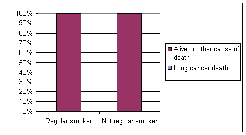
(b) Cohort study since identified and followed the explanatory variable groups and observed the resulting response.

(c) .005 - .00047 = .0046, a very small difference

(d) RR = (.005/.00047) = 10.64, OR = 10.77 (will be some rounding differences)

(e) Don’t have to rely on memory, can see how health changes over time, all patients are healthy to begin with

(f) Same as before, could be other differences about those who smoke

(g) Yes

(i) .002386, .0045, 10.7, 10.7

(j) Bars look much more similar, .5, .0045, 1.009, 1.018

Risk is not as dramatic and the RR and OR are similar.

(k).56, .4, 2, 6

Baseline is similar but now a bigger difference and the odds ratio and relative risk are not similar to each other.

(l) approximately 0, approximately 1

Are less likely to have died from lung cancer than to be in the other response variable category but the rate of lung cancer death is essentially the same between the two groups.

(m) The difference in the proportions could be the same in different tables but the odds ratio and relative risk can tell a different story. This arises based on how different the baseline risk is from .5 (when the conditional proportions are close to 0 or 1, the relative risk and odds ratio will appear more extreme and will be closer to each other in value than when the baseline risk is close to .5). When the conditional proportions are similar, both the odds ratio and relative risk will be close to 1.

Investigation 1-4: Near-Sightedness and Night Lights

(a) ou = children; variables = eye condition (categorical) and light condition (categorical)

(b) EV = lighting, RV = eye condition

(c) cross-classified since both variables were recorded about each child simultaneously

(d)

	Room light	Night light	Darkness	Total
Far-sighted	12	39	40	91
Normal	22	115	114	251
Near-sighted	41	78	18	137
Total	75	232	172	479

(e)

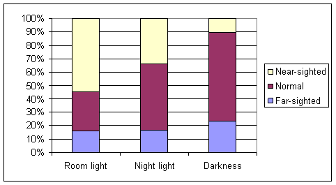
The occurrence of myopia (near-sightedness) appears to increase as the amount of light in the child’s room increases.

(f) .286, .55, .336, .105, .16, .168, .232

About 29% of children were near-sighted, but this proportion increased to .55 for the children with a room light, but was only .105 when no lighting was used. The occurrence of hyperopia was fairly constant with a slightly increased proportion among children who slept in darkness.

(g) Could be other causes such as genetics, other child-rearing issues that are related to both the type of lighting used and the eye condition of the children.

Investigation 1-5: Graduate Admissions Discrimination

(a) men: .445, women: .252

(b) Yes, men were accepted to these Berkeley graduate programs at a much higher rate than women.

(c) program, gender, whether accepted

(d) .619, .059, .824, .070

(e) the issue is that women applied more often to the program that was harder to get into overall.

(f) (108/449)(.824) + (341/449)(.070) = .25

(g) [825(.619)+373(.059)]/1198 = .44

(h)

	Program A	Program F	Total
Accepted	27	86	113
Denied	81	255	336
Total	108	341	449

(i) The weighted average is equal to the average of the two acceptance rates between the two programs.

(j)

	Program A	Program F	Total
Accepted	70	43	113
Denied	154	182	336
Total	224	225	449

(k) The weighted average is equal to the average of the two acceptance rates between the two programs.

Investigation 1-6: Foreign Language and SAT Scores

(a) EV = foreign language study (categorical); RV = SAT verbal (quantitative)

(b) Possibilities include ambition, overall academic achievement, verbal ability. For example, maybe those who take a foreign language are more likely to be interested in attending college and therefore study harder for the SAT.

(c) Randomly assign students to take a foreign language or not

(d) Want the two groups to be as similar as possible.

Investigation 1-7: Have a Nice Trip

(a) This would be a problem as gender would be confounded with the recovery strategy employed. If one group did better you wouldn’t be able to decide whether it was the strategy used or their gender.

(b) Want everything about the two groups to be as similar as possible.

(c)-(d) Results will vary

(e) Difference won’t always be zero but distribution should be centered around zero and should be equally likely to be positive as negative.

(f)-(g) Results will vary.

(h) Distribution should again center around zero.

(i) Center: 0, Largest: around .67, smallest: around -.67

(j) No, but most randomizations produce a difference that is close to zero

(k) Yes, as seen by the distribution being centered around zero

(l) Yes, as seen by the distribution being centered around zero

(m) Yes, as seen by the distribution being centered around zero

(n) Answers will vary but does seem tricky to force individuals to study certain subjects and especially to smoke or not.

(o) Power of suggestion can influence how well they do.

(p) Could assign the other group to take more English classes without telling them why, could give people cigarettes that do not contain tobacco? (Debatable)

Investigation 1-8: Have a Nice Trip

(a) Make sure you have the same number of men and women in the two groups

(b) Equal

(c) The difference in proportions will always be zero, by your design.

(d) Should be less variation than when didn’t block on gender

(e) Since height is related to gender, by making the groups more similar with respect to gender, will also be more similar with respect to height.

(f) This time, the distributions look pretty similar. Presumably gender is not related to either of these two variables.

Investigation 1-9: Friendly Observers

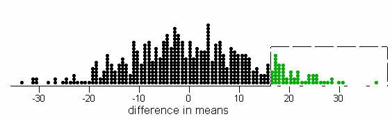
(a) The subjects were assigned to group A or group B and were not told how the two groups were being treated differently. Since the response variable (score on game) was measured objectively, there is not really a subjective rater who should be blind to group membership.

(b) EU = subjects, var1 = vested interest or not (categorical, EV), var 2 = beat threshold or not (categorical, RV)

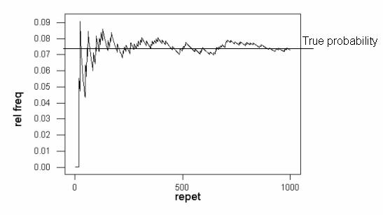
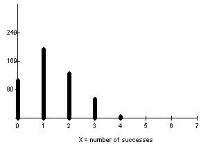
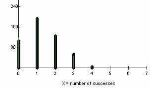
(c) .25, .67, 6

(d)

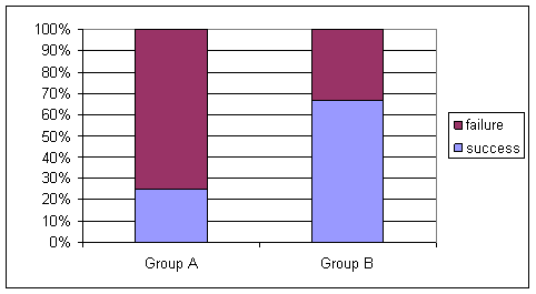
(e) .25-.67 =-.42

We observe a smaller proportion of successes (threshold beaters) in Group A (observer with vested interest) as conjectured by the researchers.

(f) Yes, randomization may not have completely balanced out the variables in the two groups and the difference we are seeing could be based on some of these extraneous variables and not on the observer’s interest level.

(g)-(j) Answers will vary

(k) 5 or 6, half of the 11 total

(l) somewhat

(m) somewhat

(n) yes, since it would be very unlikely to be a product of an “unlucky” randomization (as judged by the dotplot, a result this extreme is unlikely to happen the randomization process alone)

(o) results will vary

(p) example results

(r) About 5.5

(s) about .05

(u) some evidence since it’s unlikely to get that few successes in Group A when there really is no difference between the two groups.

Investigation 1-10: College Committee Formation

(a)-(c) Results will vary.

(d) Most likely: 0, least likely: 2, average around 2/3

(e) Answers will vary

(f) To increase the precision of the estimates, we would want to do more randomizations

(h) Answers will vary

(i) Answers will vary but should see a similar pattern as before. These results should be more “precise.”

(j) Most: 2, least: 0

(k) It is rather surprising as you should find it does not occur very often as a product of the randomization process alone.

(l) Example results:

(m) Appears to be converging to around .07.

(n) Should be converging to around 2/3.

(o) AB, AC, AD, AE, AF, BC, BD, BE, BF, CD, CE, CF, DE, DF, EF

(p) 15

(q) 1/15

(r) 1/15 = .067

(s) Should be similar

(t) 8/15, 6/15

(u) 1/15+8/15 = 9/15

(v) 6!/(2!4!) = 15

(w) C(6,3) = 20

Investigation 1-11: Selecting Senators

(a) 0, 1, 2, 3, 4, 5

(b) Calls for prediction.

(c) C(100,5) = 75,287,520

(d) C(14,1) = 14

(e) Also need to randomly decide which men will be on the subcommittee

(f) C(86,4) = 2,123,555

(g) 29,729,770

(h) P(X=1) = .395

(i) P(X=2) = C(14,2)C(86,3)/C(100,5) = .124

(j) P(X=x) = C(14,x)(86,5-x)/(100,5)

(k) P(X=x) = C(r,x)C(100-r, 5-x)/C(100,5)

(l) P(X=x) = C(r,x)C(N-r, 5-x)/C(N,5)

(k)

0	1	2	3	4	5
.463	.395	.124	.018	.001	.000

(l) sum to one

(m) E(X) = .70 = 5(14/100)

(n) 0, which is not equal to the expected value

(o) P(X=3, 4, 5) = P(X=3)+P(X=4)+P(X=5) = .0188

(p) Larger as it will be more unlikely to get an “unusual” mix

(q) P(X=2, 3) = .0484+ .002251 = .051

Investigation 1-12: More Friendly Observers

(a) 2,704,156; no

(b) P(X=3) = C(11,3)C(13,9)/C(24,12) = .0436

(c) .00582, .00032, .0000048

(d) .0498

(e) Rather unlikely to occur as a result of the randomization process alone

(f)

	Group A	Group B	Total
Beat threshold	6	16	22
Did not beat threshold	18	8	26
Total	24	24	48

(g) 6/24 = .25; 16/24 = .67

(h) Would look identical

(i) prediction

(j) Let X = number of successes in Group A. Want P(X< 6) = .0042

(k) This p-value is quite a bit smaller and provides much stronger evidence that the experimental results did not happen by chance alone.

Investigation 1-13: Minority Baseball Coaches

(a)

	Minority	Not minority	Total
1^st base	15	15	30
3^rd base	6	24	30
Total	21	39	60

X = number of minorities at 3^rd, want P(X< 6) = .015

This p-value is small enough to convince us that these results would not arise from a chance mechanism alone.

(b) This was an observational study (since race was not imposed by the researchers) so we can’t conclude “cause-and-effect” but we can say that the race and base position variables appear to be related.

CHAPTER 2

Investigation 2-1: Anticipating Variable Behavior

Answers will vary but should be justified, e.g., the number of possible distinct outcomes, the shape of the distribution, the perceived variability in the distribution, the frequency of the category corresponding to the value of zero…

Investigation 2-2: Cloud Seeding

(a) This is an experiment since the researchers imposed the seeded/unseeded condition on the clouds (the experimental units).

(b) EV = whether or not seeded (categorical); RV = volume of rain (quantitative)

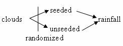
(c) Randomization was used so that the characteristics of the cloud groupings would be as similar as possible prior to imposing the treatment.

(d) To prevent any hidden “bias” that could creep into the pilots’ behavior or those making the measurements. Seems less of an issue in this context, but doesn’t hurt.

(e) The seeded clouds show a slight tendency for larger volumes of rainfall. The distribution is centered at a slightly higher value and has more of the extreme results (e.g, 1600 and above).

(f) unseeded: min = 1.0, Q₁ = 24.4, median = (41.1+47.3)/2 = 44.2, Q₃ = 163, max = 1202.6

seeded: min = 4.1, Q₁ = 92.4, median = (200.7+242.5)/2 = 221.6, Q₃ = 430, max = 2745.6

All values are in units of acre-feet.

(g) The seeded clouds have higher values for all 5 numbers in the five-number summary indicating a tendency for larger amounts of rainfall.

(h) 1.5(430-92.4) = 506.4

92.4-506.5 < 0, no low outliers

430+506.4=936.

Any clouds with more than 936.4 acre-feet of rainfall are outliers. There are four such outliers.

(i) Show min at 4.1, box from 92.4 to 430 with line at 221.6, whisker to 703.4 and then outliers at 978, 1656, 1697.8, and 2745.6.

(j) The boxplots show graphically that the distribution of the seeded clouds is shifted slightly to the right from the unseeded clouds. The box is also wider indicating more variability in the rainfall volumes.

(k) Asks for prediction

(l) The means are larger than the respective medians.

(m) 6 out of 26 (23%) in both cases. This indicates that the mean is not falling in the “middle” of the distribution as the median would

(n) possibly not as well as the median which is guaranteed to be “in the middle” of all the data values.

(o) Using Minitab:

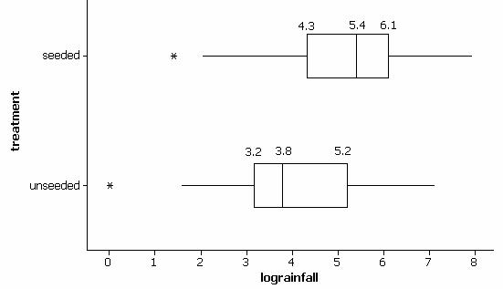
(p) The spreads of the distributions (as judged by the width of the boxes and the whiskers themselves) are more similar, and the shapes are slightly more similar (both a bit more symmetric).

(q) Yes, the seeded clouds show a higher tendency for log(rainfall) as well.

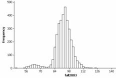
Investigation 2-3: Geyser Eruptions

(a) This is an observational study since the researchers did not randomly impose the year on some eruptions, but observed the eruptions as they occurred.

(b) Also transposing the variables, the boxplots are:

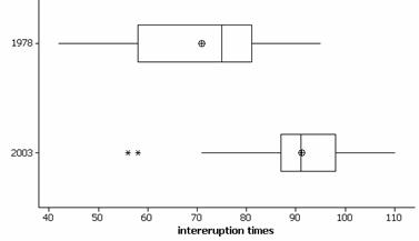
These boxplots show a tendency for longer intereruption times in 2003 as the box is shifted to the right and the lower quarter of 2003 is still above the upper quartile of 1978.

(c) Yes since the boxwidth (the interquartile range) is smaller in 2003, this is evidence that the times are less variable/more consistent. There are 2 outliers in 2003 of unusually short intereruption times for that year.

(d) 1978: 95-42 = 53; 2003: 110-56 = 54 minutes.

(e) new 2003 range = 39, much smaller than before.

(f) No, because based on (e), the range appears to be highly sensitive to outliers in the data set.

(g) From Minitab: 1978: 23; 2003: 11

(h) yes, 2003 has a smaller interquartile range so it appears to have more consistent times. Smaller spread corresponds to smaller IQR.

(i) minutes²

(j) 1978: 12.97 minutes; 2003: 8.46 minutes

(k) smaller spread corresponds to a smaller standard deviation value.

(l) new SD = 6.87, new IQR = 11.

The IQR hasn’t changed but the SD is now almost 2 minutes smaller.

(m) These approximations should be read from the graph and five number summary. About 25% of the 1978 intereruption times were less than 60 minutes compared to all but 2 of the 2003 values. Similarly, 50% of 1978 eruptions were less than 75 minutes, and even less than 25% of the 2003 eruptions were.

(n) Histograms:

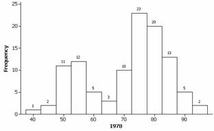
We get roughly the same percentages as above.

(o) Both the histograms (especially 1978) do reveal a bimodal shape that was hidden in the boxplot display.

The distribution of intereruption times is bimodal. The second, very short, peak is around 60 minutes.

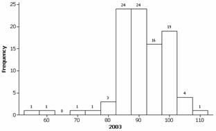
(p)

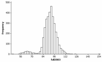
This histogram is also bimodal with a peak around 60 minutes and a much larger concentration of intereruption times around 85-105 minutes. There are a few extreme outlying times below 50 minutes and around 154 minutes.

Investigation 2-4: Bumpiness, Variety, and Variability

(a)-(d) Asks for prediction.

(e)

	Class A	Class B	Class C	Class D	Class E	Class F
Q1	3.5	2	3	1	1	6
Q3	6.5	8	7	9	9	8
IQR	3	6	4	8	8	2

Class A has the least variability of A-C. Class D has more variability than class C. Based on the IQR, Class D and E have the same variability. Class F has the least variability of all.

(f) This results are consistent, with Class F having the least, then class A. Here we do see a difference between classes D and E, with D having a slightly smaller standard deviation.

Investigation 2-5: Body Temperatures

(a) Calls for personal opinion.

(b) Could look at dotplots, boxplots, or histograms.

With dotplots:

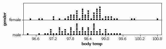
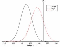
We see that both distributions are rather symmetric, with the females appearing to have a slight tendency for higher body temperatures. The mean body temperature for the females in this sample is 98.394 degrees compared to 98.105 degrees for the males (median 98.4⁰ vs. 98.1⁰). The female body temperatures also show slightly more variability (SD=.743 degrees vs. .699 degrees, though the IQR has .8 for the females and 1.0 for the males). If we look at the boxplots, we see that the larger standard deviation for the females arises in large part from about 5 outliers.

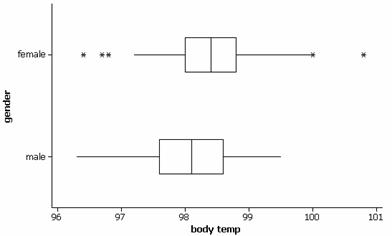
(c) A temperature of 98.6^o appears rather typical for the females but is close to the upper quartile (98.6) for males. Would be nice to know the conversion between the Fahrenheit and Celsius scales to answer the second question.

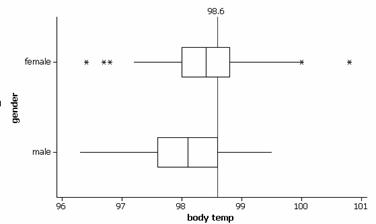
(d) female: (98.6-98.394)/.743 = .277

male: (98.6-98.105)/.699 = .708

(e) With a higher z-score, a temperature of 98.6⁰ is “further” above the male average than the female average.

(f) female: (98-98.394)/.743 = -.53

male: (98-98.105)/.699 = -.15

A temperature of 98⁰ appears to be more unusual for the females since the absolute value of the z-score is larger.

(g) A negative z-score indicates the observation lies below the mean.

(h)

	Mean	Standard dev
Female	36.885	.413
Male	36.725	.388

(i) The new mean is (5/9)(98.395-32) for the women and (5/9)(98.105-32) for the men, transformations of the means on the Fahrenheit scale. For the standard deviations, we use just the scale term: (5/9)(.743) and (5/9)(.699).

(j) (5/9)(98.6-32) = 37

(k) female: z = (37-36.885)/.413 = .28

male: z = (37-36.725)/.388 = .71

These are the same (apart from some rounding discrepancies) as the z-scores obtained on the Fahrenheit scale.

(l) 0

(m) 68%

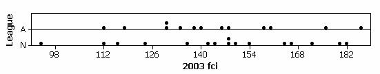
Investigation 2-6: The Fan Cost Index

(b)

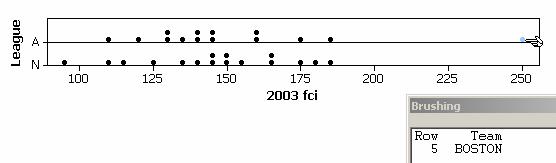
(c)

Boston is again identified as an outlier.

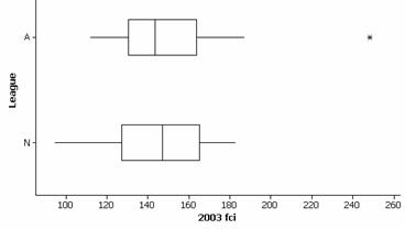
(d) The five number summary (in dollars) and mean/SD are below.

Variable League Minimum Q1 Median Q3 Maximum

2003 fci A 112.02 130.37 143.69 163.73 248.44

N 94.61 127.32 147.32 165.11 182.56

Variable League Mean StDev

2003 fci A 151.92 34.60

N 145.81 24.88

(e) The costs are rather similar in that there is much overlap of the boxes and while the median FCI value is slightly higher for the National League, the mean American League FCI value is higher. The standard deviation for the American League is slightly larger though the IQR is slightly lower ($33.36 vs. $37.79). Both distributions appear fairly symmetric.

(f) American; National; The FCI for Boston is pulling the mean up.

(g) National; American; The FCI for Boston is also inflating the standard deviation.

(h) Calls for predictions.

(i)

Now Montreal might be flagged as a low outlier for the National League FCI values. The mean AL FCI value is now down to $145.22 with standard deviation $23.02. These are now a bit below the NL mean and standard deviation values, agreeing with the comparison we would draw if we focused on the median and IQR.

(j) Median since it is calculated based on the position of the observations and not their numerical values. An extreme numerical value will always affect the calculation of the mean.

(k) The IQR since it is calculated based on the position of the observations and not their numerical values. An extreme numerical value will always affect the calculation of the standard deviation and the range..

(l)

mean=$3.45, sd = $8.93, median = $2.13, IQR = $13

The distribution of price differences is fairly symmetric, centered near zero, but with a fairly large spread. If we compare the two leagues:

There is much more variation in the differences for the American League than the National League (SD $11.08 vs. $6.88, IQR $15.76 vs. $11.35). Both distributions center around 3 dollars, although the median AL difference is much closer to $0.

(m) Largest percentage change: Anaheim

Largest 2003 FCI: Boston

Largest change: Boston 19.71, Texas -19.79

While Boston raised their FCI value by almost $20, it was already one of the highest (2002: $228.78) so it was a smaller fraction. Anaheim only raised their FCI value by $16.44 but since they started at $113.76 this is a larger percentage change. Anaheim won the World Series in 2002 so a jump in prices the following year is not all that surprising.

(n) Also shifting to a more sensible scale:

These prices tend to occur at integer values. This makes sense as they are often sold by vendors walking the stands and it is more convenient to not have to make change.

(o) There is a $4.08 program (Montreal) value and two $10.2 cap values (Montreal and Toronto).

(p) They are the Canadian teams and the prices have been converted to US dollars. These values are probably integers in Canadian dollars.

(q) No

(r) They are not all actually the same size.

(s) Montreal is unusually low and Boston is unusually high.

Investigation 2-7: House Prices

(a) Answers will vary but should look for a “typical” value.

(b) Answers will vary but could look at the “prediction” errors.

(c) answers will vary

(d) ideally zero!

(e) 582.5

(f) 4660-8m = 0 yields m = 582.5

(g) mean = 582.5, median = 507

the mean balances all of the prediction errors.

(h) Sx_i – nm = 0 yields m = Sx_i/n

(i)-(k) answers will vary

(l)

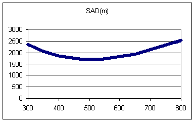
The shape appears parabolic in nature but is piecewise linear.

(m) Any value between 469 and 545, inclusive, leads to an SAD of 1716, the smallest possible.

(n) These values fall between the 4^th and 5^th ordered data values. The cut-offs are precisely the 4^th and 5^th values.

(o) While the graph moves to higher values overall, the minimizing flat spot occurs at the same values of m.

(p) Now the flat spot ranges from 529 to 545, what are now the 4^th and 5^th values.

(q) calls for conjecture but if only 9 values in the data set, it appears we want a value between the 4^th and 5^th values, inclusive.

(r) The function y values will be scaled but the minimum will be achieved by the same values of m.

(s)-(t) answers will vary

(u)

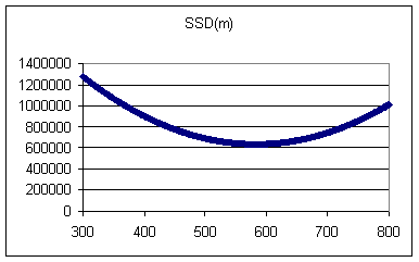
This function is a concave up parabola. The function is minimized between m = 582 and 583 (and should be halfway in between).

(v) Now the function is minimized between m = 682 and 683. This is a rather dramatic effect whereas the minima of the SAD did not change.

(w) The mean of the data set.

(x) m = Sx_i/n

(y) SSD changed more and the mean changed more.

(z) The mean takes into account all of the individual numerical values whereas the median relies only on positioning.

(aa) Calls for opinion but might worry about a “typical” value like the median that won’t be inflated by a few very expensive homes.

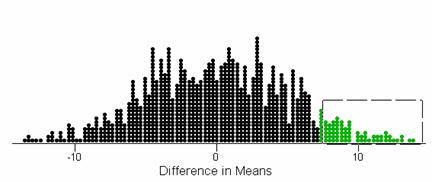
Investigation 2-8: Sleep Deprivation and Visual Learning

(a) Experiment since the subjects were assigned to either get sleep the first night or not.

(b) EV: sleep (categorical); RV: performance score (quantitative)

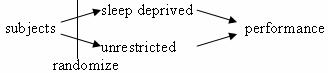
(c) The unrestricted group tended to have larger improvement values than the sleep deprived group. In fact, only one member of the unrestricted group failed to improve where as 3 of the deprived group decreased in performance by a fairly large amount.

(d) means: 15.92 medians: 12.05

(e) Yes, by chance.

(f)-(h) results will vary

(i) Calls for judgment based on where the observed difference in means falls in the distribution.

(j) Results will vary.
(k) Example results

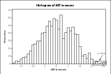
(l) Results will vary, probably less than .01.

(m) Since we get a difference between the group means as large as 15.92 in less than 1% of randomizations by chance alone, this provides strong evidence that there is some other difference between the two groups.

(n) Since this was a randomized experiment, we can attribute the difference between the two groups to the sleep deprivation on that first evening.

(o) C(21,11) = 352,716

(p) Distribution looks similar.

(q) 2533/352716 = .0072, should be close to the simulated p-value.

Investigation 2-9: More Sleep Deprivation

(a) The variability in performance scores as exhibited by the widths of the boxes.

(b) Calls for prediction.

(c)-(d) Example results:

p-value » .112, much larger than for the actual experiment.

(e) These hypothetical data provide much less evidence of a significant difference between the two groups. With the larger variation within the groups, the difference in group means observed does not appear as surprising.

Investigation 2-10: Lifetimes of Notables

(a)

	Minimum	Lower quartile	Median	Upper quartile	Maximum
Writers	29	60	66	78.5	90
Scientists	48	62.5	76	86.5	94

(b) The lifetimes of the scientists tend to be longer (every number in the five number summary is larger and the mean is lifetime is 73.25 compared to 66 years for the writers). The lifetimes of scientists also tend to be more variable (IQR = 24 vs. 18.5 years) though the writers do have a few more of the extreme low values (standard deviations are more similar at 14.18 years for the scientists and 16.57 years for the writers). The distribution for the writers has a slight skew to the left while the distribution of these scientists appears a bit more symmetric.

(c) This was an observational study. The researchers did not impose the occupations on these subjects.

(d) Example results:

p-value » .06, .07

The randomization distribution is symmetric around zero and the observed difference in means of 7.25 occurs less than 10% of the time.

(f) While there is some evidence it is not extremely strong. If we used 5% as our “cut-off” value, then we would not say the observed difference in means was statistically significant.

(g) No, since this was an observational study we cannot conclude that the occupation is what led to the difference in mean lifetimes observed between these groups.

CHAPTER 3

Investigation 3-1: Sampling Words

(a) Results will vary.

(b) Length of word is quantitative and whether or not the word is “long” is categorical.

(c) We suspect that the samples will tend to overrepresent the longer words.

(d) Results will vary but the observational units are the words and the horizontal axis should be labeled “length” or “number of letters” or such.

(e) Results will vary but the observational units are the words.

(f) statistic since it is calculated for a sample,

(g) proportion since it is calculated about a sample,

(h) parameter, m

(i) 99/268 = .369, parameter, p

(j) no, no

(k) Results will vary, we suspect that a large percentage of the observations will lie above 4.29.

(l) Results will vary, we suspect that a large percentage of the observations will lie above .369.

(m) results will vary

(n) results will vary

(o) No, the sampling method will tend to overrepresent the longer words. We see evidence of this in the fact that the distribution lies to the right of the parameter value instead of being centered around the parameter value.

(p) No, longer words will still have a higher probability of being landed on.

(q) Assigning each word a number and randomly selecting the numbers.

(r) 268, 3 digits

(s) results will vary

(t) results will vary but the distributions should not center around the parameter values.

(u) no; no; now centered at the parameter value

(v) should be about half

(w) yes

Investigation 3-2: Comparison Shopping

(a) The observational units are the produces, the sample are the 30 items selected, the population is all products common to both stores (or all the items on the inventory list).

(b) Number the items from 01 to N = number of items on the inventory list and then randomly choose 30 numbers and find the corresponding products on the inventory list.

(c) Will take some time to find the products in the stores.

(d) A little easier to get the list of 30 items but will still take time to find them in the store.

(e) Randomly select a sample of items, then in each aisle, flip a coin to decide right or left, then randomly select a shelf, and then number all the 2 foot sections and randomly select a two foot section.

(f) Yes, through the sampling method we know exactly where the items are located.

(g) No since items that take up more shelf space or more likely to be selected.

(h) Yes, yes since they are a different type of item and a store may choose to “specialize” in one of these but not both with respect to cheaper prices.

(i) Number all of the food items, 1 to N, and then randomly select 22 products. Then number all of the non-food items, 1 to M, and then randomly select 8 products.

Investigation 3-3: Sampling Variability of Sample Means

(a) Population = all words in the Gettysburg address; Sample = 5 words selected; Sampling Distribution = distribution of the sample means resulting from all possible random samples of size 5 from this population.

(b) C(268, 5) = 1.11´10¹⁰

(c) Population is skewed the right. The mean is m = 4.29 letters and the standard deviation is 2.12 letters.

(d) Results will vary.

(e) Results will vary.

(f) Results will vary. Probability is 1/(1.11´10¹⁰).

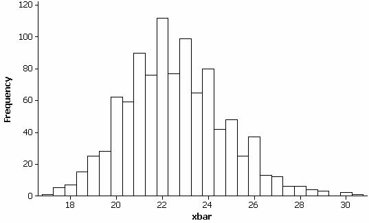
(g) (₁ + ₂)/2 should equal the value displayed by the red arrow.

(h) observational units are the samples, the variable is the sample mean, the shape is slightly skewed to the right, the center should be around 4.29 letters, the standard deviation should be around 1 letter. There may be 1 or 2 visual outliers. For example:

(i) The different simulations should all lead to very similar pictures.

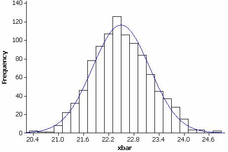
(j) The distribution of sample means should be less skewed and less spread out, with center still around 4.29 letters. For example:

(k) Yes

(l) Can try to visually judge from the graph what percentage of sample means are larger. Probably won’t be too many.

(m) Yes, there are very few sample means above 6 in the above simulation.

(n) No, a sample mean of 4.8 is closer to the mean of the sampling distribution.

(o) This would be even less surprising with the smaller sample size. In fact, Scott’s 6.7 has 2 or 3% of samples falling above it.

(p) n=10: Scott: z » (6.7-4.29)/.65 = 3.71; Kathy: z » (4.8-4.29)/.65=.785;

n = 5: Scott: z » (6.7-4.29)/.99 = 2.43; Kathy: z » (4.8-4.29)/.99 = .52

Scott with n = 10 has the largest z score.

Investigation 3-4: Sampling Variability of Sample Proportions

(a) Since they are random samples, the results should be unbiased and the sample proportions should center around the population proportion p = .369. The distribution of sample proportions is the sampling distribution.

(b) The distribution will be less spread out if the samples are larger.

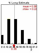
(c) The sampling distribution should appear skewed to the right with a mean of approximately .37 and a standard deviation around .22. For example:

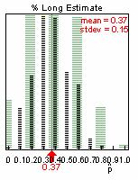
(d) The shape should appear more symmetric, with a mean of approximately .37 and a standard deviation around .15. For example:

(e) C(268, 5) = 5.42´10¹⁴ so the probability of any particular sample occurring is 5.42´10^-14. Since there are 99 long words in the population, there are C(99,5) = 71,523,144 samples containing 5 long words.

(f) .0064

(g) Yes, we are selecting a random sample from a finite population of successes (long words) and failures (short words).

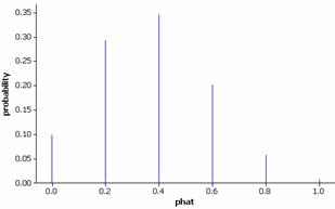
(h) The distribution appears slightly skewed to the right and should look very similar to the empirical sampling distribution.

(i) E(X) = .369, which is the same as the center of the empirical sampling distributions.

(j) When n = 10

(k) E(X) = .369

(l) The exact and empirical sampling distributions should be very similar.

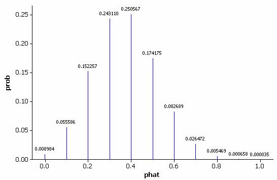
(m) The distribution is less skewed and less spread out but has the same center.

(n) P( = 1) = .000035. This is much smaller than the probability in (f) as it is even less likely to find all long words in a sample of 10 than in a sample of 5.

(o) Hypergeometric with N = 268, M = 50, and n = 10

x P( X <= x )

1 0.413559

This would not be a surprising outcome.

(p) Hypergeometric with N = 268, M = 50, and n = 10

x P( X <= x )

4 0.977636

So P(X>5) = 1-P(X<4) = 1-.9776 = .0224. This small probability indicates that it would be a bit surprising to obtain a sample with 5 or more nouns if only 18.7% of the words in the population were nouns.

Investigation 3-5: Freshman Voting Patterns

(a) The observational units are the freshmen, the variable is whether they planned to vote for Kerry or Bush (categorical).

(b) The sample is the 30 respondents, the population is the 705 first-years on campus, and the sampling frame is the list of residence halls, and then the rooms within the residence halls.

(c) This was a multistage systematic sampling plan since they randomly chose dorms, then rooms within dorms (every 7^th room). This method should be unbiased but since they only selected one dorm they do need to be cautious that students in that dorm do not feel tremendously different on this issue than students in the other dorms (which seems like a plausible belief).

(d) The surveys were anonymous and confidential and the names of the candidates were rotated.

(e)

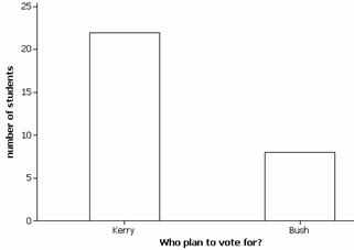
The sample reveals that most students (73%) planned to vote for Kerry.

(f) Hypergeometric with N = 750, M = 352, and n = 30

x P( X <= x )

21 0.997414

The probability of 22 or more freshmen indicating Kerry, if 50% of the population planned to vote for Kerry, would be 1-.9974 = .0026. This indicates that about .26% of samples would yield a result this extreme if Kerry and Bush were equally preferred in the population. This provides strong evidence that the claim about the population is incorrect.

(g) Hypergeometric with N = 750, M = 500, and n = 30

x P( X <= x )

21 0.718464

The probability of 22 or more freshmen indicating Kerry, if two-thirds of the population planned to vote for Kerry, would be 1-.7185 = .2815. This indicates that about 28% of samples would yield a result this extreme if two-thirds of the population plan to vote for Kerry. Thus, such a sample result would not be surpring.

(h) It appears to be more plausible that p = 2/3 than .50.

Investigation 3-6: Comparison of Sampling Methods

(a) The population of prices is skewed to the right with mean $2.58 and standard deviation $1.44.

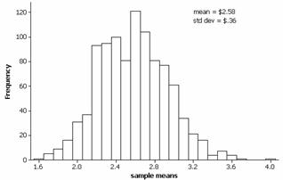
(b) Macro:

sample 14 c2 c4

let c5(k1)=mean(c4)

let k1=k1+1

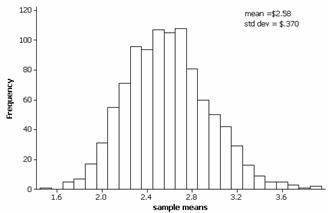
The distribution of sample means is slightly skewed to the right with mean $2.58 and standard deviation $.37.

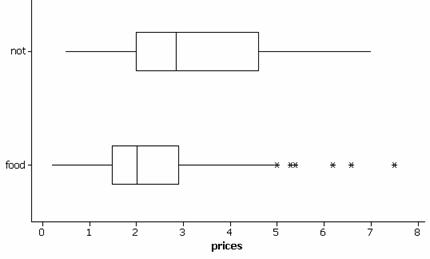
(c) There are 40 non-food items and 104 food items so that 72% of products are food items.

(d) There is a tendency for the non-food items to be more expensive (mean $3.14 versus $2.36).

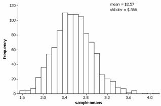
(e) Macro commands:

sample 4 c6 c8

sample 10 c7 c9

stack c8 c9 c10

let c11(k1)=mean(c10)

let k1=k1+1

The distribution of sample means has a teeny right skewness. The mean is $2.59 and the standard deviation is $.357.

This distribution appears very similar to the one in (b).

(f)

(g)

Investigation 3-7: Do Pets Looks Like Their Owners?

(a) Answers will vary

(b) If just guessing, the probability is 1/3 that will match the correct pet with this owner.

(c) Would be the same for everyone.

(d) No, the responses are independent.

(e) Y has a Bernoulli distribution with p = 1/3. P(Y=1) = 1/3 and P(Y=0) = 2/3.

(f) Answers will vary.

(g) Answers will vary.

(h) 1(1/3) + 0(2/3) = 1/3. Should be similar.

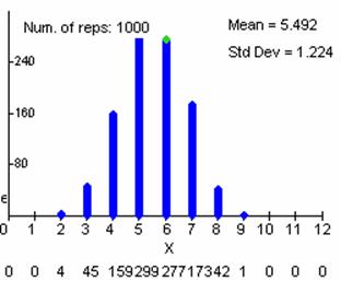
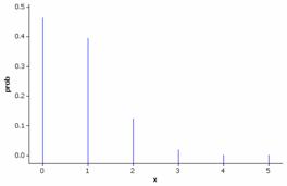
Investigation 3-8: Pop Quiz!

(a) Answers will vary.

(b) Answers will vary.

(c) Success = answering the question ‘correctly’

Failure = not matching the stated answer.

p = ¼ for all 5 questions

the responses to the questions are independent

(d) X = 0, 1, 2, 3, 4, 5

X will vary from person to person

(e) Answers will vary

(f) number of students with one correct / total number of students

(g) Results will vary. For example:

(h) No, guessers are more likely to get 0, 1, or 2 correct answers than 3 or 4.

(i) There are 32 possible arrangements.

(j) No since we are more likely to get a failure than a success, outcomes like FFFSS are more likely than outcomes like SSSFF.

(k)

SSSSS SSSSF SSSFS SSFSS SFSSS FSSSS

5 4 4 4 4 4

SSSFF SSFSF SFSSF FSSSF SSFFS SFSFS FSSFS SFFSS FSFSS FFSSS

3 3 3 3 3 3 3 3 3 3

FFFSS FFSFS FSFFS SFFFS FFSSF FSFSF SFFSF FSSFF SFSFF SSFFF

2 2 2 2 2 2 2 2 2 2

FFFFS FFFSF FFSFF FSFFF SFFFF FFFFF

1 1 1 1 1 0

(l) P(FFSFF) = (3/4)⁴(1/4) = .0791

(m) No, are 5 ways to have just 1 success

(n) All 5 outcomes with 1 success have probability .0791 of occurring.

(o) P(X = 1) = 5(.0791) = .3955

(p) P(2 successes) = (1/4)²(3/4)³ = .0265

P(X = 2) = 10(.0265) = C(5,2)(.0265) = .2637

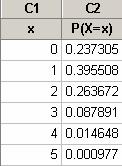
(q)

Number of correct answers, x	0	1	2	3	4	5
Probability, P(X=x)	0.237305	.3955	.2637	0.087891	0.014648	0.000977

(r) Since all of the probabilities are nonnegative and they sum to one, this is a legitimate probability distribution.

(s) They should be similar.

(t) P(X = x) = C(n, x) p^x(1-p)^n-x for x = 0, 1, 2, …, n

(u) Binomial with n = 5 and p = 0.25

x P( X = x )

1 0.395508

(v)

(w)

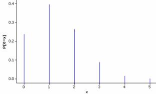
The graph is skewed to the right with a peak at x=1. E(X) = 1.25 indicating that if we were to average the number of correct answers over many many trials, the average will converge to 1.25 correct answers.

(x) P( > .5) = P(X > 3) = 1 – P(X < 2)

Binomial with n = 5 and p = 0.25

x P( X <= x )

2 0.896484

The student will get 3 or more correct answers with probability 1-.8965 = .1035.

(y) P( > .5) = P(X > 8) = 1- P(X< 7)

Binomial with n = 16 and p = 0.25

x P( X <= x )

7 0.972870

The student will get 8 or more correct answers with probability 1-.9729 = .0271.

This probability is smaller. If someone is just guessing, we expect them to get the correct answer 25% of the same. Getting “lucky” and getting more than 50% correct answers should be less likely as we decrease the number of questions. We more questions, the relative frequency of correct answers should get closer and closer to .25.

(z) P(X < k-1) > .95

Binomial with n = 15 and p = 0.25

x P( X <= x ) x P( X <= x )

6 0.943380 7 0.982700

If we choose the 7, the P(X < 7) > .95 and P(X > 8) < .05.

This corresponds to = 8/15 = .533.

Investigation 3-9: Water Oxygen Levels

(a) water samples

(b) Most like a systematic random sample with the observations coming at fixed intervals in time.

(c) The sample should be representative of the river during this time. Might be a little cautious a bout generalizing to too broad a period of time.

(d) Yes, if we consider p to the be the probability of a non-compliant measurement and we are assuming the measurements are independent.

(e) p < .10

(f) C is counting the number of successes with a fixed probability of success (p = .10) for a finite number of independent trials (n = 10).

(g) = 4/10 = .40, statistic

(h) Yes, this proportion could differ from .10 by random chance.

(i) E(X) = 10(.1) = 1 day

The sample result (4 days) is larger than the expected result which is the direction conjectured by the researchers (more non-compliant days)

(j) P(C > 4) = 1- P(C< 3)

Binomial with n = 10 and p = 0.1

x P( X <= x )

3 0.987205

P(C > 4) =1-.9872 = .0128

It is rather surprising (probability .0128) to find a sample of 10 days with at least 4 non-compliant days if we are sampling from a process with p = .10.

(k) P(C > 3) = 1- P(C< 2)

Binomial with n = 10 and p = 0.1

x P( X <= x )

2 0.929809

P(C > 3) = 1 - .9298 = .0702.

This is also surprising but not as surprising. If we use .05 as a cut-off value this would not be convincing evidence of a problem.

(l) P(C > 19) = 1- P(C< 18)

Binomial with n = 34 and p = 0.1

x P( X <= x )

18 1.00000

P(C > 19) = 1- 0 » 0

It would be virtually impossible to find 19 or more non-compliant days if we are sampling from a process with p = .10. This provides very strong evidence that p > .10 for this river at this time.

Investigation 3-10: Heart Transplant Mortality

(a) Could consider the heart transplantation process at this hospital.

(b) p = the probability of a heart transplantation resulting in death at this hospital

(c) p = .15

(d) p > .15

(e) H_o: p = .15, H_a: p > .15

(f) = 8/10 = .80 which is indeed larger than .15.

(g) We have success (death) and failure (not death) for a fixed number of trials (n=10) where we are assuming the probability of success is constant (p = .15) for the 10 independent measurements (outcome of one patient does not affect the probability of success for the next patient).

(h) E(X) = np = 10(.15) = 1.5 deaths

(i) P(X > 8) = 1- P(X< 7)

Binomial with n = 10 and p = 0.15

x P( X <= x )

7 0.99999

P(X > 8) = 1- .99999 = .00001

(j) It is very surprising to find 8 or more deaths with sampling from a process with p = .15. We would expect such a result in .001% of samples from this process.

(k) P(X > 71) = 1- P(X < 70)

Binomial with n = 361 and p = 0.15

x P( X <= x )

70 0.990303

P(X > 71) = 1-.9903 = .0097

(l) With a p-value below .01 we would reject the null hypothesis and conclude that p, the probability of a death, is higher than .15 for this hospital.

Investigation 3-11: Do Pets Looks Like Their Owners?

(a) Since the outcomes (success = match owner with dog) for the 28 judges will be independent and everyone has a .5 probability of guessing correctly, X will be binomial with n = 28 and p = .5.

(b) P(X > 15) = 1- P(X < 14)

Binomial with n = 28 and p = 0.5

x P( X <= x )

14 0.574723

P(“match”) = 1-.5747 = .4253

(c) Since the outcomes (success = group match) for the 45 owners will be independent and each owner has a .4253 probability of being matched, Y will be binomial with n = 45 and p = .4253.

(d) E(X) = 45(.4253) = 19.1 match

(e) Parameter, let p = probability of the judges matching the owner with the correct dog.

H₀: p = .4253 (probability that the panel matches the dog if just guessing)

H_o: p > .4253 (higher probability of a match than just guessing)

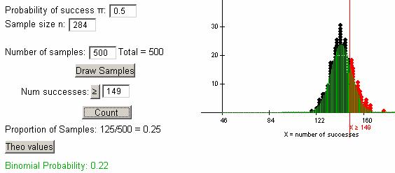
p-value = P(Y > 23) = 1 – P(Y< 22)

Binomial with n = 45 and p = 0.4253

x P( X <= x )

22 0.844587

p-value = 1-.8446 = .1554

With such a large p-value (.1554 > .05), we fail to reject the null hypothesis.

Our conclusion is that, while the judges did better than expected, they did not perform significantly better than we would expect if they were guessing randomly.

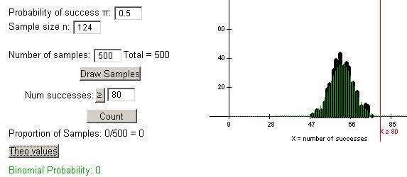
(f) p-value = P(Y > 16) where Y is binomial with n = 25 and p = .4253.

Binomial with n = 25 and p = 0.4253

x P( X <= x )

15 0.974944

p-value = 1-.9749 = .0251

At the .05 level of significance, p-value < .05, so we can reject the null hypothesis.

There is convincing evidence at the 5% level that the judges were able to correctly match more of the pure-bred dogs than we would expect by chance if they were just guessing.

Investigation 3-12: Halloween Treat Choices

(a) The observational units are the treat or treaters. The variable of interest is which treat they choose (categorical, possible outcomes = toy or candy).

(b) Let p = probability of a child choosing the toy (arbitrarily treating a toy as a success)

(c) p = .5 (null)

(d) would expect half or 142 of the children to choose the toy

(e) 135 is fewer children than expected

(f)

(g) 135 is 7 below the expected 142

(h) P(X > 149):

(i) two-sided p-value = .44, this is not statistically significant at the .05 level.

Investigation 3-13: Kissing the Right Way

(a) The observational units are the kissing couples and the population appears to be all kissing couples in these public areas in these countries (and perhaps even broader). Since there was nothing special about how the couples were identified, we can consider this a representative sample of the kissing in public process.

(b) If we assume the behavior of the couples are independent and that the probability of success (turning to the right) is constant across the couples (helped by not having them dealing with luggage etc.) then X is binomial with n = 124 and p = probability of kissing couple turning to the right.

(c) H₀: p = .5 (equally likely to turn right and left)

H_a: p ≠ .5 (not equally likely) – answers will vary

(d) H₀: p = .5 (equally likely to turn right and left)

H_a: p > .5 (more likely to turn to the right)

p-value » 0

With such a small p-value we will reject the null hypothesis.

There is strong evidence that couples are more likely to turn to the right than to the left.

(e) H₀: p = 2/3 (2/3 of couples will turn to the right)

H_a: p ≠ 2/3 (the probability of turning to the right differs from 2/3)

p-value = .633.

We would fail to reject H₀.

The probability of turning to the right is not significantly different from 2/3.

Investigation 3-14: Kissing the Right Way (cont.)

(a) Best guess would be 80/124 = .645

(b) While we think p should be close to the observed proportion of successes, we know due to sampling variability that it is probably not exactly .645.

(c) The largest value of p is .72

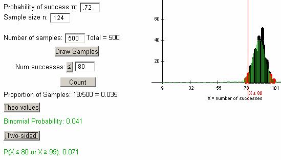
The smallest value of p is .56

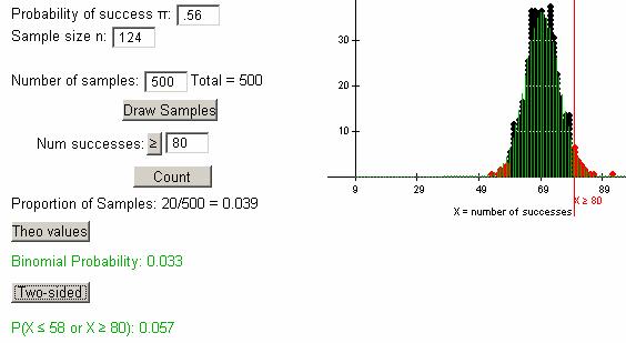
Any value of p between (including) .56 and .72 lead to two-sided p-values above .05.

(d) More values of p would now “qualify.”

(e) Exact

Sample X N Sample p 95% CI P-Value

1 80 124 0.645161 (0.554230, 0.728983) 0.002

Minitab reports a 95% confidence interval from about .55 to .73.

(f)

Test of p = 0.667 vs p not = 0.667

Exact

Sample X N Sample p 95% CI P-Value

1 80 124 0.645161 (0.554230, 0.728983) 0.634

(g)

Test of p = 0.5 vs p > 0.5

95%

Lower Exact

Sample X N Sample p Bound P-Value

1 80 124 0.645161 0.568368 0.001

Investigation 3-15: Improved Batting Averages

(a) H_o: p = .250 (player is still a .250 hitter)

H_a: p > .250 (player is trying to show his average has increased)

(b) X is binomial since the at-bats will be independent, there are 20 of them, and we are assuming the probability of success (getting a hit) is the same for every at bat.

(c) There is a fair bit of overlap in the two distributions indicating that it is difficult to tell a .250 hitter and a .333 hitter apart in 20 at-bats. The player could have a tough time demonstrating his improvement.

(d) X > 9

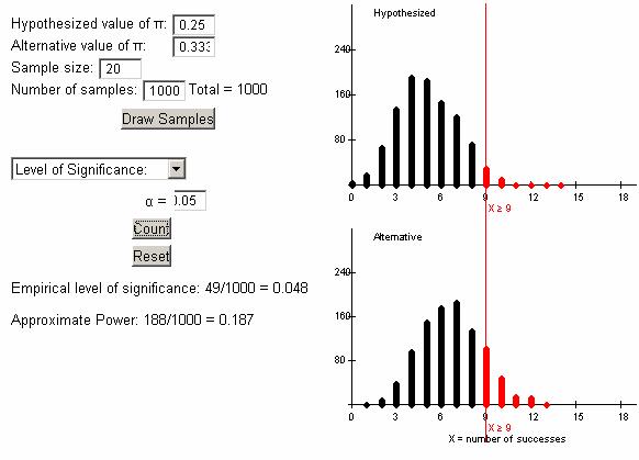
(e) .048

(f) .187

(g) Need x < 8 or x > 9

(h) P(X > 9) = 1- P(X < 8)

Binomial with n = 20 and p = 0.333

x P( X <= x )

8 0.810338

1-.8103 = .1897 (very similar to the applet value)

(i) If the player gets 7 hits, this is less than 9, so the manager would not be convinced of the player’s improvement. This is a mistake since the player is actually a .333 hitter.

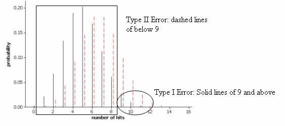
(j) Type I Error: Think the player has improved when he has not

Type II Error: Think the player has not improved when actually he has

(k) P(Type I Error) » .048

P(Type II Error) = .81

(l) power = 1-.81 = .19

(m) The player would prefer the type II error has a small probability (failing to see his improvement). The owner would prefer the type I error has a small probability (falsely thinking the player has improved).

(n) To reduce the probability of a Type I error, we need to raise the standard for improvement to 10.

(o) empirical level of significance (prob of type I error) is down to .016 and probability of a type II error is now 1-.083 = .917

(p) more at-bats

(q) yes, as the unimproved player will be less likely to get “lucky” and the improved player will be less likely to get “unlucky”

(r) The distributions are now more clustered around their own respective means.

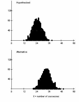
(s) Rejection region: X > 34

(t) Type II error = 1-.449 = .551, much smaller than before, and power = .449, much larger than before.

(u) Yes, there is now a higher probability that the player will be able to demonstrate that improvement.

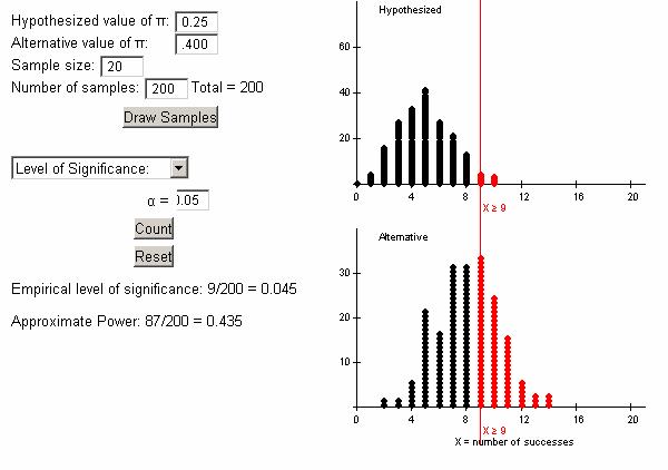
(v) Rejection region: X > 37

probability type II error = .785

this change helped the manager but hurt the player

(w) should be easier to demonstrate that he is not a .250 hitter.

(x) Less overlap in the distributions.

P(Type I Error) still about .045

P(Type II Error ) = .565, less than in (k)

(y)

(z) If P(Type I Error) decreases, then P(Type II Error) increases and vice versa. But the owner prefers small P(Type I Error) while the player prefers small P(Type II Error). The level of significance controls P(Type I Error). Increasing the sample size and increasing the alternative probability away from .250 both decreased P(Type II Error).

Investigation 3-16: Sampling Words (cont.)

(a) 99/268 = .369

(b) yes, yes

(c) 98 long, 169 short

(d) P(also long) = 98/267 = .367, this is reasonably similar to the previous probability

(e) P(5^th also long) = 95/264 = .3598

(f) not hugely different

(g) 49/218= .225, now we are looking different.

(h) Yes since 268 > 20(5) = 100, n = 268, p = .369

(i)

Binomial with n = 5 and p = 0.369

x P( X = x )

5 0.0068412

This probability, .0068, is close to the exact probability .0064.

(j) Yes since 268 > 20(10) = 200.

(k)

This probabilities look pretty similar.

(l)

Row x binom hyper

5 4 0.000003 0.000000

6 5 0.000015 0.000003

7 6 0.000064 0.000015

8 7 0.000234 0.000070

9 8 0.000737 0.000271

10 9 0.002011 0.000900

11 10 0.004821 0.002576

12 11 0.010251 0.006412

13 12 0.019483 0.013998

14 13 0.033303 0.026969

15 14 0.051470 0.046087

16 15 0.072238 0.070163

17 16 0.092408 0.095499

18 17 0.108078 0.116565

19 18 0.115871 0.127910

20 19 0.114122 0.126447

21 20 0.103442 0.112801

22 21 0.086417 0.090932

23 22 0.066615 0.066308

24 23 0.047424 0.043772

25 24 0.031199 0.026171

26 25 0.018975 0.014176

27 26 0.010669 0.006957

28 27 0.005546 0.003092

29 28 0.002664 0.001244

30 29 0.001182 0.000453

31 30 0.000484 0.000149

32 31 0.000183 0.000044

33 32 0.000063 0.000012

34 33 0.000020 0.000003

35 34 0.000006 0.000001

36 35 0.000002 0.000000

Not looking so similar any more.

Investigation 3-17: Feeling Good

(a) sample of adults in the US

(b) population is people in the US

(c) answers will vary, parameter

(d) the same as the answer to (c)

(e) yes since the US population is much larger than 20(1017)

(f) Answers will vary depending on guess and direction of H_a. Should use the binomial approximation.

(g) Type I Error: Thinking the population proportion is larger/smaller/different than my guess when it actually isn’t.

Type II Error: Thinking the population proportion is equal to my guess when it is actually larger/smaller/different.

If you rejected H₀, then it’s possible are committing a Type I Error. If failed to reject H_o, is possible are committing a Type II Error.

(h) Values between .858 and .899 would not be rejected.

(i) Exact

Sample X N Sample p 95% CI P-Value

1 895 1017 0.880039 (0.858472, 0.899377) 0.000

We are 95% confident that between 85.8% and 89.9% of American adults feel good about the quality of their life overall. If you rejected your guess, then it would not be contained in the confidence interval.

Investigation 3-18: Long-term Effects of Agent Orange

(a) observational study since they didn’t randomly select which people to the agent orange.

(b) residents of Bien Hoa City

(c) No but assume it’s rather large

(d) Yes if the population in (b) is much larger than 43

(e) H₀: p = .5 (half of residents have elevated levels)

H_a: p > .5 (more than half of residents have elevated levels)

Test of p = 0.5 vs p > 0.5

95%

Lower Exact

Sample X N Sample p Bound P-Value

1 41 43 0.953488 0.860731 0.000

With such a small p-value (< .001) we have very strong evidence to reject H₀ and conclude that more than half of all current residents in Bien Hoa City have elevated levels of TCDD.

(f) If p = .5, that would indicate that the median was equal to 5 ppt.

CHAPTER 4

Investigation 4-1: Pot Pourri

(a) All of the distributions are reasonably symmetric without many outliers.

(b) The center and spread differ across the distributions.

(c) Same shape but vertical axis has been scaled.

(d) The total area represented is one.

(e) It has some resemblance to the overall pattern.

(f) The normal probability curve provides a reasonable model for all 8 variables.

Investigation 4-2: Body Measurements

(a) The normal distribution provides a reasonable model for these data.

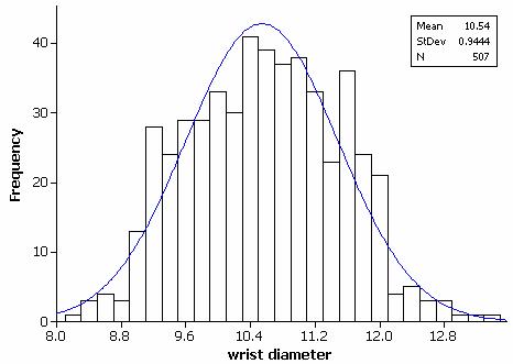
(b)

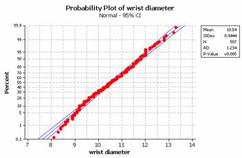
(c) The small wrist diameters appear to deviate slightly from the linear pattern. This is also seen by those bar heights being consistently lower than the normal curve in the histogram.

(d) The graphs indicates that the lower weights are smaller than we would expect them to be (shorter left tail).

(e) The graphs indicate that the smaller diameters are even smaller than we would expect them to be (a longer left tail).

(f) The graphs indicate two mounds in the distribution, perhaps due to gender differences.

(g) The genders look fairly normal when graphed separately. The female girths appear slightly skewed to the right. The male girths show a very slight skew to the left.

(h)-(i) The histograms should all look reasonably normal and the normal probability plots should look reasonably straight (large p-values).

(j) It will be difficult to judge the shape in the histograms with such small samples, but the normal probability plots should still look roughly linear, but with lots of variation.

Investigation 4-3: Fuel Capacity

(a) mean = 16.38, std dev = 2.708

(b) Between 16.38-2.71 and 16.38+2.71 = 13.67 and 19.09

(c) 74/108 or 68.5% of the values are in this range as predicted by the empirical rule (68%)

(d) estimates will vary

(e)

Normal with mean = 16.38 and standard deviation = 2.708

x P( X <= x )

13 0.105987

probability = .106

(f) If we were to repeatedly sample cars from this population, we would find a fuel capacity below 13 gallons about 10.6% of the time.

(g) 11/108 or 10.2%

Investigation 4-4: Body Measurements (cont.)

(a) Answers will vary

(b) Yes, both appear reasonably normal but they differ in the centers of the distributions.

(c) A height of 185 would be surprising for a female but not for a male.

(d)

(f) Normal with mean = 164.9 and standard deviation = 6.55

x P( X <= x )

185 0.998925

(g) The total area under the curve is one and P(X>185) = 1-P(X< 185) = 1-.9989 = .0011.

(h) 1- P(X<185) = .8454 = .1546

ormal with mean = 177.7 and standard deviation = 7.18

x P( X <= x )

185 0.845355

(i) z (female) = (185-164.9)/6.55 = 3.07

z (male) = (185-177.7)/7.18 = 1.02

The female z-score is higher than the male z-score as a height of 185 is further from the female mean than the male mean.

(j)-(l) Both distributions look reasonable normal with mean 0 and standard deviation 1.

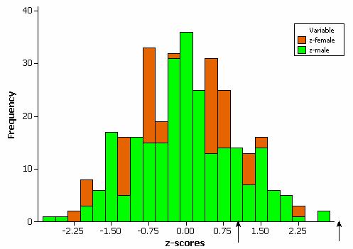
(m) 1-.9987 = .0013

(n) 1-.8461 = .1539

These are essentially the same (just differ due to rounding)

(o) z=(151.8-164.9)/6.55 = -2.00

prob below » .02275

(p) .02275 corresponds to a z of about -2.00. To be at least 2 standard deviations below the mean, a male would have to be 177.7-2(7.18) = 163.3 cm or shorter.

(q) z = -2.00 in both.

Investigation 4-5: Birth Weights

(a)

ßweights à ßweights à

Center is at 3250, label: weights

(b) within one sd of mean, 3250-550 = 2700 and 3250 + 550 = 3800

(c)

ßweights à

z = -1.36

prob = .0863

A baby of low birth weight is 1.36 standard deviations below the mean. If we repeatedly sample babies from this population, in the long-run, 8.63% of babies will be of low birth weight.

(e) 291154/3880894 = .075, slightly below the value predicted by the normal distribution

(f)

ßweights à

(g) applet: z=2.34, prob = .0097

(h)

ß weights à

(i) z = -.45 and 1.36, prob =.5889

(j) 2552852/3880894 = .66, not as close but in the ball park.

(k)

(l) z = -1.96, weight = 2172 grams.

(m)

z = 1.96, weight = 4328 grams.

These two weights are both about 2 standard deviations from the mean.

(n)

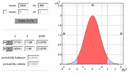
Between 2716 and 4282 grams.

(o) Again the z-scores are -1.96 and 1.96.

Investigation 4-6: Reese’s Pieces

(a) Yes, we are counting the number of successes (orange candy) in a fixed number (25) of independent trials.

(b) No, the actual outcome of X will vary from student to student.

(c) Statistic, results will vary.

(d) Results will vary

(e) No

(f) Should be symmetric, with mean near 11-12.

(g) Yes, with mean about 11-12 and standard deviation about 2.5.

(h) The horizontal axis would scale so the center is around .45-.50 and the standard deviation is around .1.

(i) The actual values of will probably differ but the applet will report the average of the values of that you obtain.

(j) shape should be pretty symmetric, center should be around .45, std dev should be around .1

(k) Should match fairly well.

(l) 68%, 95%, 99.7%

(m) answers will vary

(n) should be fairly close

(o) less variable

(p) normal model still appropriate, std dev now much smaller, above 90% will be within + .10.

(q) predictions will vary

(r) will now center around .65

(s) more spread out. Might also notice that the normal approximation is no longer all that reasonable.

Probability Theory Detour

(a) E(X) = np = 25(.45) = 11.25

(b) 11.25/25 = .45

(c) E(X/n) = (1/n)E(X) = (1/n)(np) = p

(d) SD() = SD(X/n) = (1/n)SD(X) = (1/n)

(e) E() = .45

SD() = .0995

(f)

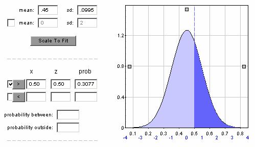
ß sample proportions à

(g) mean = .45, std dev = sqrt(.45*.55/75) = .0574

P( > .75):

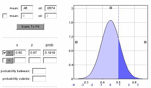
ß sample proportions à

This probability is much smaller as we would expect the sample proportion to be closer to .45 with the larger sample size.

(h)

The sample proportion will be between .35 and .55 in about 92% of samples.

Investigation 4-7: Cohen v. Brown University

(a) observational units: students; population/process: determination of athletes and non-athletes; parameter: p = probability of a Brown University intercollegiate athlete is female.

(b) H₀: p = .51 (probability that an athlete is female is the same as the proportion of female at Brown)

H₀: p < .51 (women are underrepresented among the athletes)

(c) Check n p = 897(.51) = 457.5 > 10 and n(1-p)=897(.49)=439.5 > 10 and, since we are treating this as a random sample, the conditions for the Central Limit Theorem to apply are ment.

(d) z = (.38-.51)/sqrt(.51*.49/835) = -7.79 so that the observed sample proportion is almost 8 standard deviations below the conjectured value.

(e)

ß sample proportion à

The p-value is very small.

(f) We have very strong evidence that the small sample proportion did not result by chance from a process with p = .51. The sample proportion is significantly lower than .51.

Investigation 4-8: Kissing the Right Way (cont.)

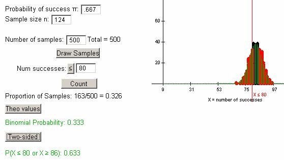
(a) With n = 124 and p₀ = 2/3, we have np =124(2/3) = 82.7 and n(1-p) = 124(1/3) = 41.3. If we consider this a random sample then the Central Limit Theorem applies.

(b) SD = .0423

ß proportion of sample turning to right à

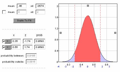
(c) z = (.65 - .667)/.0423 = -.40

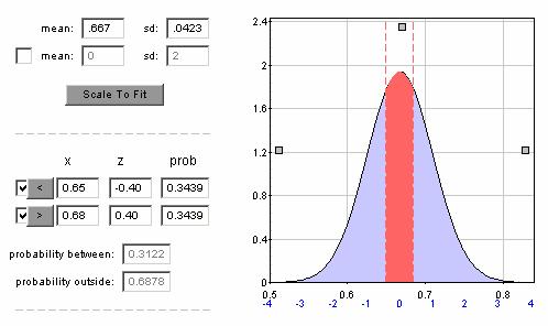
We want the probability outside: .6878.

We fail to reject H₀ at the 5% level.

We do not have significant evidence that p differs from .667.

(d) This two-sided p-value is fairly similar to what we obtained before.

(e) A test statistic of -.40 indicates that the observed sample proportion (.65) is .4 standard deviations below the conjectured value of .667.

(f)

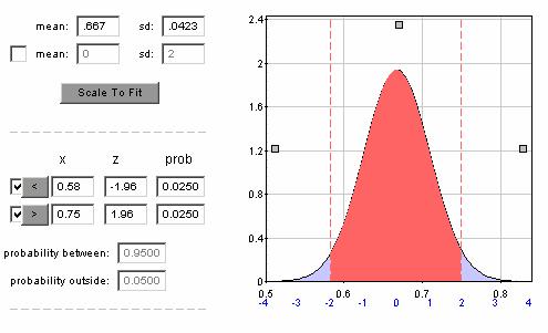
For the two-sided p-value to be below .05, we need the test statistic to be approximately -1.96. This corresponds to a sample proportion of .667 – 1.96(.0423) = .58

(g) .667 + 1.96(.0423) = .76

(h)

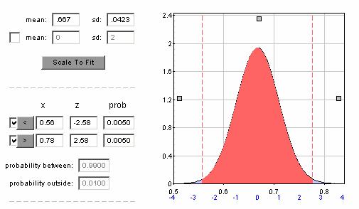
Now need to be 2.58 standard deviations from the mean, .558 - .776. These cut-offs are more extreme as expected as the lower level of significance requires more extreme evidence.

(i) .05, type I

(j) If p = .5, the sampling distribution of the sample proportion will be centered at .5 with standard deviation .0449. So we need to find P( < .584) . Note P( > .750) » 0.

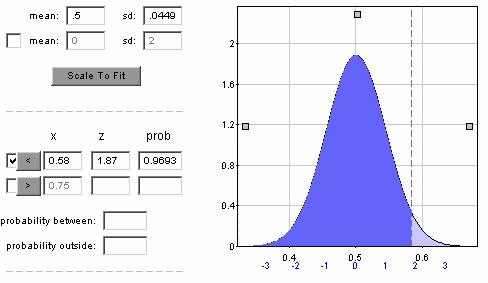
So the probability is .9693 that will fall < .584 and we will reject H₀: p = 2/3.

(k) .01, type I;

P( < .558 or > .750 when p = 2/3) = .01

P( < .558 when p = .5) = .9018. This is smaller than before.

(l) If we increase alpha, power increases.

If we increase the sample size, power increases

If we use .6 instead of .5, the power will decrease as it will be harder to reject p = 2/3 in favor of .6 than in favor of .5.

(m) Assuming a 5% level of significance, the cut-off (rejection region) is found by going 1.96 standard deviations below 2/3. The P(Type II Error) is then found by seeing how many standard deviations this cut-off is above .5. We want the cut-off to be about 2.33 standard deviations above .5.

.5+2.33sqrt(.5*.5/n) = .67 – 1.96sqrt(2/3(1/3)/n)

= 2.089/.17 = 12.3

n > 152

Investigation 4-9: Cohen v. Brown University

(a) Should be within two standard deviations of p.

(b) within 2 standard deviations.

(c) use

(d) sqrt(.38(.62)/897) = .0162

(e) .38 – 2(.0162) and .38 + 2(.0162) = .348 and .412

(f) .975

(g) 1.96

(h) .38 + 1.96(.0162) = .348 and .412

(i) .51 is not in this range (we rejected .51 as a plausible value for p earlier).

(j) We are 95% confident that the process at Brown University leads to between 34.8% and 41.2% of athletes being female.

(k) z* = 2.576

.38 + 2.576(.0162) = .38 + .042 = .338 - .422

This interval is wider than the 95% confidence interval.

Sample X N Sample p 95% CI Z-Value P-Value

1 341 897 0.380156 (0.348389, 0.411923) -7.18 0.000

Sample X N Sample p 99% CI Z-Value P-Value

1 341 897 0.380156 (0.338407, 0.421905) -7.18 0.000

Investigation 4-10: Reese’s Pieces

(a) Results will vary for + 1.96 .

(b) Not everyone in class will obtain the same interval.,

(c) May even be a few in class that do not have .45 in their interval. We don’t expect this method to work every time.

(d) Results will vary. If the interval is green, .45 is contained in the interval. Otherwise the interval will be red.

(e) Will probably not get the same exact interval both times.

(f) The population proportion did not change but is represented by a fixed vertical line in the “graph”.

(g) Results will vary but the running total should be somewhere near 95%.

(h) The running total should hover around 95%.

(i) The red intervals correspond to the smallest and largest values.

(j) Predictions will vary.

(k) The intervals reduce in length. The running total should hover around 90%.

(l) No.

(m) This probability will correspond to the confidence level.

(n) Either the interval contains p or it does not, so we would not assign a probability to the interval containing p. We can do this before we observe the sample and generate the interval, but not after.

(o) Conjectures will vary.

(p) The intervals are less wide.

(q) Conjectures will vary.

(r) The intervals will shift to be around .65 but the coverage rate wills till be around 95%.

Investigation 4-11: Good News or Bad News First

(a) Bar graph should have one bar for good news and one for bad. Results will vary.

(b) Let p = proportion of all students at your school that prefer bad news first. Interval calculation will vary but interpretation will be that you are 95% confident that the interval captures p.

(c) Probably do not pass np >10 and n(1-p)>10.

(d) Coverage rate will be around 80%, not close to the 95% confidence level.

(e) Probably at least 95%.

(f)-(g) Calculations and summary will vary.

(h) Probably not, do you feel the statistics class is a representative sample of all students at your school?

Investigation 4-12: Scottish Militiamen and American Moms

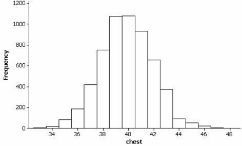
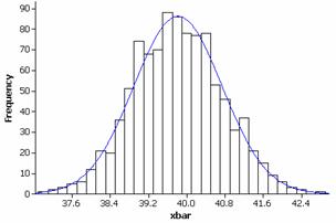
(a) observational units = militiamen, variable = chest measurement (quantitative)

(b) The distribution of chest measurements for early 19^th century militiamen appears symmetric with mean 39.8 inches and standard deviation 2.05 inches. If we are considering this our population, we have calculated m and s.

(c) Results will vary. For example:

The shape will be difficult to judge with only 5 observations, the sample mean should be in the ballpark of 39.8 inches and the sample standard deviation should be in the ballpark 2.05inches. These are parameters and we could denote them by and by s.

(d) The observational units are samples and the variable is the sample mean. Results will vary but the distribution of the sample means should be symmetric with mean near 39.8 and standard deviation near .9. For example:

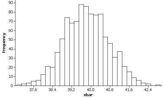
The distribution has a similar shape and center as the population but is less variable.

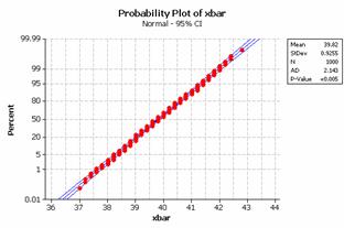
(e) The normal distribution does appear to be a reasonable model, e.g.,

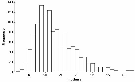
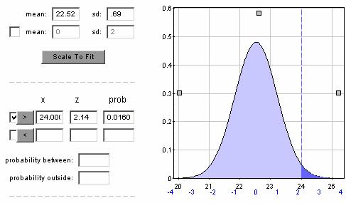
(f) The distribution of ages for this sample of mothers is skewed to the right with mean m = 22.52 and standard deviation s = 4.885

(g) Results will vary but the distribution of the sample means is less skewed than the population, with mean near the population mean of 22.52 and standard deviation of about 2.2. For example:

(h) Conjecture will vary.

(i) Results will vary but this distribution should be reasonably modeled by a normal distribution with mean near the population mean of 22.52 years and standard deviation of about .7 years. For example:

(j) This distribution is more symmetric and has less variability than the distribution with samples of size n-5.

(k)

Population	Shape	Center	Standard deviation
Normal m=39.8, s =2.05, n=5	Symmetric	39.6 (m)	.92 smaller than s
Skewed m = 22.52, s=4.89, n=5	Slight skew to right	22.5 (m)	2.2 smaller than s
Skewed m = 22.52, s=4.89, n=50	Symmetric	22.52 (m)	.69 much smaller than s

(l)

Population	s/	Simulation
Normal m=39.8, s =2.05, n=5	.92	similar
Skewed m = 22.52, s=4.89, n=5	2.2	similar
Skewed m = 22.52, s=4.89, n=50	.69	similar

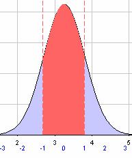
(m) P(> 41) = .10

Distribution of sample means will be normal with mean = 39.83 and standard deviation .92.

(n) Distribution of sample means will be symmetric with mean 22.52 years and standard deviation 4.89/sqrt(50) = .69 years.

(o) No, since the distribution of sample means is not predicted to be well modeled by the normal distribution.

(p) We can still conjecture that the probability will be larger since the standard deviation will be larger, 4.89/sqrt(5) = 2.2 indicating that it would be less surprising to obtain a sample mean this far from the population.

Minitab Exploration: Confidence Interval for m

(a) + z* s/.

(b) Results will vary but percentage should be close to 95%.

(c) The percentage will be less than 95%, closer to 88-90%.

(d) For example:

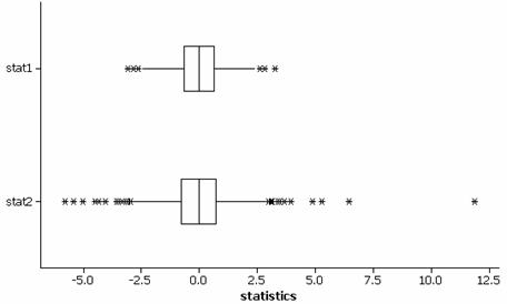
The distribution of stat1 is less variable, with shorter tails, than the distribution of stat2.

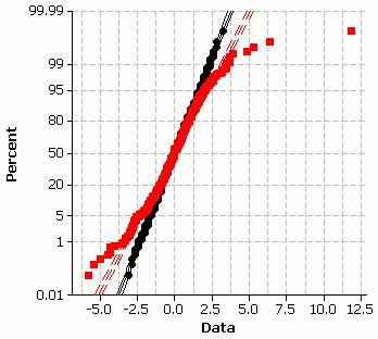
(e) The distribution of stat1 (in black) appears to be well modeled by a normal distribution but not the distribution of stat2. The normal probability plot also reveals the longer tails in the distribution of Stat2.

(f) t* = 2.776, z* = 1.96, the t critical value is larger.

(h) The percentage should now be close to 95%.

(i) Yes, since, in the long-run, 95% of intervals succeed in capturing the value of the population mean.

Applet Explorations

Exploration 1

(a) no, more like 84%

(b) yes, near 90%

(c) coverage rate of z with s intervals should be between 88-90% and coverage rate of t-interval is near 90%

(d) Extreme values (large or small) of lead to intervals that fail to capture m.

(e) No, since the width also depend on s which changes from sample to sample.

(f) The t procedures are preferred since the coverage rate will be close to the claimed coverage rate.

Exploration 2

(a) Sampling distribution is approximately normal as is the sample distribution. The latter is much more variable.

(b) Yes

(c) The sampling distribution is approximately normal and the distribution of the sample is skewed to the right. The sample has a shape similar to that of the population but the Central Limit Theorem indicates that the sampling distribution of sample means will be normal for n=50. Approximately 90% of the intervals will capture m.

(d) The sampling distribution will still be fairly symmetric and the distribution of the sample will still be skewed. The coverage rate will probably be a bit below 90%.

With n=5, the sampling distribution will be skewed and the coverage rate will be way below 90% (about 80-85%).

(e)-(g) The coverage rate will still closer to 90%, even for n=5 since the population distribution is symmetric to begin with.

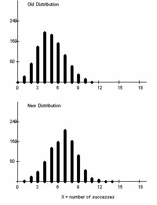
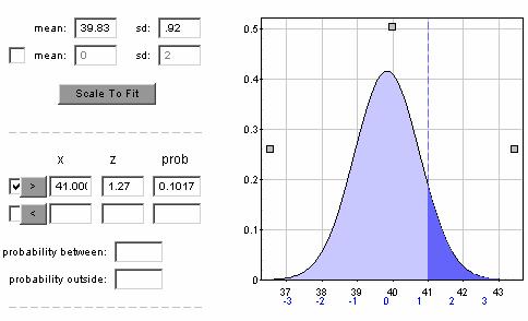
Investigation 4-13: Basketball Scoring

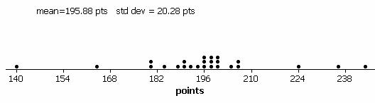
(a) The distribution of total points scored is fairly symmetric with mean = 195.88 pts and standard deviation s = 20.27 points.

(b) Let m = average total points scores per game after the rule change.

H₀: m = 183.2 (scoring did not increase)

H_a: m > 183.2 (scoring is higher on average)

(c) standardize the observation

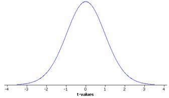
(d) The sampling distribution of the test statistic would be well-modeled by a t distribution with 24 degrees of freedom.

(e)-(f) n= 25 but since the sample is reasonably symmetric, it is plausible that the population distribution follows a normal distribution.

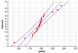
(g) Not really, these observations were recorded during the same three day period near the beginning of the season. This time period may not be representative of the season as a whole as players are still getting into playing shape and may still be adjusting to the new rule changes.

(h) t₀ = (195.88-183.2)/(20.27/sqrt(25)) = 3.13

estimates will vary

(i) 1- .9977 = .0023, the p-value

(j) With a p-value < .05, we would reject the null hypothesis and conclude that the average points scored per game this season is higher than 183.2. However, we have some doubts as to the validity of this procedure since we did not a have a random sample of games and also relies an the belief that the population distribution of points scored is reasonably symmetric.

(k) t = 1.71

195.88 + 1.71(20.27/sqrt(25)) = (188.9, 202.8)

We are 90% confident that the mean points scored per game this season is between 188.9 points and 202.8 points. We cannot conclude that the rule changed caused the increase in scoring since this was an observational study.

(l) 13/25 à 52% of games fall in this interval, not close to 90% but that is not what the 90% confidence level claims

(m) No, in fact, an even smaller percentage since the interval will be narrower with the larger sample size.

(n) = 195.88

(o) s = 20.27

(p) 195.88 + 1.71 (20.27)sqrt(1+1/25) = 195.88 + 35.35

We are 90% confident that between 160.53 and 231.23 points will be scored in a game.

(q) Wider as now we are trying to predict an individual value not just the population mean.

(r) Should be close to 90% (22/25 = 88%).

(s) Test of mu = 183.2 vs > 183.2

95%

Lower

Variable N Mean StDev SE Mean Bound T P

points 25 195.880 20.272 4.054 188.943 3.13 0.002

(t)

Variable N Mean StDev SE Mean 90% CI T P

points 25 195.880 20.272 4.054 (188.943, 202.817) 3.13 0.005

(u) 95% CI for m: 190.18, 206.91

This interval is narrower than the 90% confidence interval.

(v) t = 1.71 with p-value = .0502 or t = 1.74 with p-value = .0472

So the null hypothesis would be rejected for a t-value larger than 1.71.

Investigation 4-14: Comparison Shopping

(a) observational units = grocery store products, population = products common to both stores, sample = 29 items selected. Predictions about cheaper store will vary though are told that Lucky’s advertises itself as a discount store.

(b) This was a systematic sample.

(c)

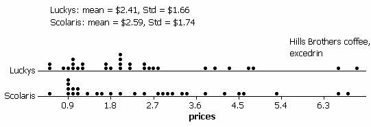
Both distributions appear skewed to the right, centered around 2.5 dollars but with similar spread. The same two products (Hill’s Brothers French Roast and Excedrin (50 tablets) appear to be outliers in both distributions.

(d) Since the same products were obtained at both stores. It makes more sense to compare the products to their counterpart at the other store.

(e) Examining the distribution of price differences.

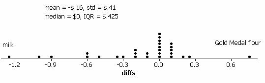
The distribution has a slight skew to the left. There is a cluster around $0 but there appears to be more products that are more expensive at Scolari’s than at Lucky’s.

(f) The outliers here are not the same as in (b). They seem to stem for the products not being exactly identical at the two stores.

(g) Yes, any where the products do not match at the two stores.

Just one item was removed, n is now 28.

(h)

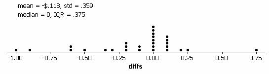
Still a small amount of evidence that there are more products that are more expensive at Scolari’s.

(i) H₀: m = 0 (no tendency for one store to be more expensive)

H_a: m < 0 (on average, higher prices at Scolaris)

(j) Test of mu = 0 vs < 0

95% Upper

Variable N Mean StDev SE Mean Bound T P

diffs 28 -0.118214 0.358774 0.067802 -0.002728 -1.74 0.046

We would reject the null hypothesis at the 10% level (p-value = .046 < .10). There is moderate evidence that, on average, Scolari’s has more expensive products.

(k)

Variable N Mean StDev SE Mean 90% CI

diffs 28 -0.118214 0.358774 0.067802 (-0.233701, -0.002728)

We are 90% confident that the average price difference is between .3 cents and 23 cents (more expensive at Scolari’s).

Investigation 4-15: Sampling Words

(a) E() = m = 4.29 and SD() = s/= 2.12/sqrt(10) = .670

(b) Since the population distribution is clearly skewed to the right and the sample size is small, we may suspect that the sampling distribution will not be well-modeled by a normal distribution.

(c) sample mean, = 4.80, sample standard deviation, s = 2.15, 95% t interval, (3.26, 6.34).

We would be 95% confident that m is between 3.26 letters and 6.34 letters.

(d) Results will vary but will probably differ from the original sample mean.

(e) Results will vary from sample to sample.

(f) Results will vary. Below are the results of one such simulation.

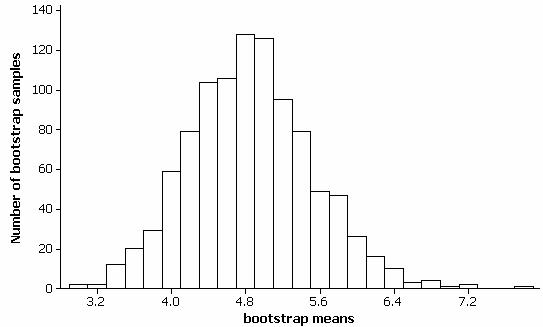
(g) Results will vary but for the above simulation, the mean of these 1000 bootstrap means is 4.81 letters and the standard deviation is .669 letters. The standard deviation should be close to the theoretical values of SD().

(h) 4.80 + 2.262(.669) = (3.29, 6.31). We would be 95% confident that m is between 3.29 letters and 6.31 letters. This interval is very similar to the t interval in (c).

(i) ^*_.975 = 6.2

(j) ^*_.025 = 3.5

(k) = 4.80

2-^*_.975 = 2(4.80)-6.2 = 3.4

2-^*_.025 = 2(4.80)-3.5 = 6.1

(l) We need to find ^*_.95 and ^*_.05 from the bootstrap distribution.

^*_.95 = 6.0

^*_.05 = 3.80

2-^*_.95 = 2(4.80)-6.0= 3.6

2-^*_.05 = 2(4.80) -3.8 = 5.8

The 90% bootstrap confidence interval would be (3.6, 5.8).

(m) Results will vary from class to class but should be similar to 90% if each student took a different random sample.

Investigation 4-16: Comparison Shopping (cont.)

(a) Below are sample results:

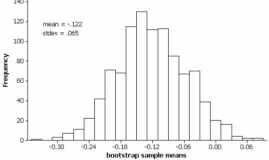
The bootstrap distribution is roughly symmetric with mean similar to the sample mean -$.118 and standard deviation approximately $.065.

(b) The 97.5^th percentile value should be around .0086 and the 2.5^th percentile should be around -.25. So the bootstrap percentile interval is

2(-.118 ) - .0086 = - .24

2(-.118) – (-.25) = .01

Investigation 4-17: Heroin Treatment

(a) The distribution is skewed to the right with a median of 367.5 days and an inter-quartile range of 418.5 days.

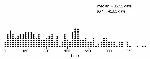
(b) An example bootstrap distribution:

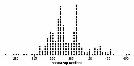
The distribution is fairly symmetric but irregular. The standard deviation is 31.55 days.

(c) The 97.5^th percentile value should be around 450 and the 2.5^th percentile should be around 323.5.

2(367.5) – 450 = 285

2(367.5) – 323.5 = 411.5

A 95% percentile bootstrap confidence interval for the population median is approximately 295-411.5 days.

(d) 25% trimmed mean for the sample is 376.5 days.

(e) An example bootstrap distribution:

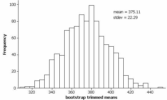
The distribution is fairly symmetric with mean near the sample trimmed mean (376.5) and standard deviation around 22.3 days.

(f) The 97.5^th percentile value should be around 421.6 and the 2.5^th percentile should be around 334.1 (or so).

2(376.5) – 421.6 = 331.4

2(376.5) – 334.1 = 418.9

A 95% percentile bootstrap confidence interval for the population trimmed mean is approximately 334.8 – 419.8 days.

CHAPTER 5

Investigation 5-1: Newspaper Credibility Decline

(a) So that there is no bias due to the order in which the choices are presented. For example, people may have a tendency to respond more negatively toward the end of the list if they are getting tired of the survey process.

(b) observational units = respondents

variable 1= believability rating of their daily newspaper

This is an observational study since we are only surveying their opinion and not imposing any treatments. The samples are the respondents in 2002 and the respondents in 1998. The populations are everyone who could rate their daily newspaper in 2002 and 1998. We could also consider the year the explanatory variable (though again, we did not randomly assign this condition to different people in the sample) and the distribution of this variable was controlled by the study design.

(c) Two-way table:

	1998	2002	Total
Largely believable	618	587	1205
Not largely believable	922-618=304	932-587=345	649
Total	922	932	1854

There does not appear to be a large difference in the sample proportions who rate their local daily newspaper as largely believable (.670 and .630) though a higher proportion felt it was largely believable in 1998 than in 2002.

(d) Yes, sampling variability.

(e) Yes if we take n=922 and p = proportion in population who would rate their paper as largely believable in 1998. This was a random sample so the trials (respondents) will be independent. The population is more than 20 times the size of the sample so we will consider the probability of success to be approximately constant for every member of this sample.

(f) Yes, for the same reasons in (e) with n=932 and p = proportion in population who would rate their paper as largely believable in 2002.

(g) No, Z does not count the number of successes and failures in a fixed number of trials.

(h) If there was no difference between the two years, then p₁-p₂ would be zero.

(i) H₀: p₁ – p₂ = 0 (no difference in the proportion who rate the paper as large believable in these two populations)

H_a: p₁ – p₂ > 0 (the population proportion in 1998 is larger than the population proportion in 2002)

Note: we are assuming p₁ represents 1998.

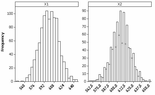
Results will vary, but the distributions should be pretty symmetric with

	X1	1	X2	2
Mean	599.3	.65	605.8	.65
Std Dev	14.48	.0157	14.56	.0156

The values in the table are the theoretical mean and standard deviation for each distribution and should be similar to the values obtained from the simulation.

(k) Both sample proportion sampling distributions would be reasonably well modeled by a normal distribution (as confirmed by normal probability plots). For ₁ we would assume mean p = .65 and standard deviation = .0157. For ₂ we would assume mean p₂ and standard deviation = .0156.

(l) Sample results are shown below

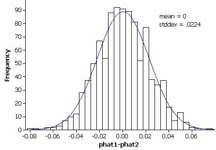
The distribution looks reasonably well modeled by a normal distribution with mean 0 and standard deviation .022.

(m) About 3 or 4% of the simulated differences were larger than .04. This would lead to a p-value below .05 and we would conclude that the difference in the sample proportions did not occur by chance alone. The difference in sample proportions is statistically significant and we can generalize these results to the 1998 and 2002 populations since the samples were selected at random. This is an observational study and not an experiment so we cannot make any causal statements as to why this decline has occurred.

Investigation 5-2: Newspaper Credibility Decline (cont.)

(a) Results will vary but should be similar to the theoretical values.

(b) E(₁ – ₂) = E(₁) – E(₂) (by rules of expected value)

= E(X/n₁) – E(Y/n₂) (by definition of )

= E(X)/n₁ – E(Y)/n₂ (by rules of expected value)

= n₁p₁/n₁ – n₂p₂/n₂ (by definition of expected value of binomial random variable)

= p₁-p₂

V(₁ – ₂) = V(₁) – V(₂) (since the samples are independent)

= V(X/n₁) + V(Y/n₂) (by definition of )

= V(X)/n₁² + V(Y)/n₂² (by rules of variance

= n₁p₁(1-p₁)/n₁² + n₂p₂(1-p₂)/n₂² (by definition of variance of binomial random variable)

= p₁(1-p₁)/n₁ + p₂(1-p₂)/n₂

(c) With n₁ = 922 and n₂ = 932, p₁=p₂=.65,

E(₁-₂) = p₁-p₂ = .65 -.65 = 0 which is the average of the simulated differences.

V(₁-₂) = p₁(1-p₁)/n₁ + p₂(1-p₂)/n₂ = .65(.35)/922 + .65(.35)/932 = .000491

SD(₁-₂) = sqrt(.000491) = .0222 which is very similar to the standard deviation of the simulated differences.

(d) test statistic possibility:

Since the sampling distribution is approximately normal, we can compare this test statistic to the standard normal distribution to obtain a p-value.

(e) = (618+587)/(922+932) = .6499

SE(₁-₂) = sqrt(.6499(1-.6499)(1/922+1/932)) = .0222

z = (.6703-.6298)/.0222 = 1.825

p-value = P(Z>1.825) = .034

The standard error is close to the simulated value and the p-value is in the ball park of the simulated value.

(f) With a small p-value (less than .05), we have strong enough evidence (at the 5% level of significance) to reject the null hypothesis and conclude that the population proportion who rate their daily papers as largely believable decreased between 1998 and 2002.

(g) SE(₁-₂) = sqrt(.6703(1-.6703)/922 + .6298(1-.6298)/932) = .0221

90% confidence interval: .6703-.6298 + 1.645 (.0221) = .0405 + .0364 = (.0041, .0769)

(h) We are 90% confident that the difference in the population proportions (p₁-p₂) is between .0041 and .0769. That is, between .4% and 7.7% fewer people rate their daily paper as largely believable in 2002 compared to 1998.

(i) If we were to repeatedly draw samples from these populations and calculate a confidence interval for the population difference each time, roughly 90% of these intervals would succeed in capturing the true difference.

(j) Yes, zero is not contained in the 90% confidence interval, consistent with rejecting the null hypothesis p₁-p₂ = 0 at the 5% level of significance.

(k) The 95% confidence interval.6703-.6298 + 1.96(.0221) = .0405 + .0433 = (-.0028, .0838)

This interval is wider than the 90% confidence interval (and in fact now includes 0 as a plausible value of the difference in the population proportions).

(l) ₁ = 619/924 = .6699 ₂ = 588/934 = .6296,

SE(₁-₂) = sqrt(.6699(1-.6699)/924 + .6296(1-.6296)/934) = .0221

95% confidence interval: .6699 - .6296 + 1.96(.0221) = .0403 + .0433 = (-.0030, .0836)

We are 95% confidence that the difference in the population proportions is between -.0030 and .0836. This interval is very similar to the Wald interval.

Minitab output:

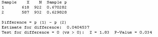
Wald:

90% CI for difference: (0.00398935, 0.0767368)

95% CI for difference: (-0.00292560, 0.0838329)

Wilson: 95% CI for difference: (-0.00297889, 0.0837051)

Investigation 5-3: Sleepless Drivers

(a) Observational units: drivers

Variables: whether had a full night’s sleep during the previous week, whether or not involved in a crash resulting in injury.

Will probably consider the sleep variable as the explanatory variable.

(b) Observational since the sleep variable was not imposed by the researchers.

(c) Case-control since they identified cases (those involved in car crashes) and controls (not involved in car crashes that resulted in injury).

(d) We can consider these as independent samples from those who obtained a full night’s sleep and those that did not.

(e) No since this is a case-control study and the proportion of drivers involved in accidents in this study was determined by the researchers.

(f) H₀: t = 1 (there is no association between sleep variable and accident variable)

H_a: t > 1 (there is a positive association, those with less sleep have higher odds of being involved in an accident)

(g)

	No full night’s sleep in past week	At least one full night’s sleep in the past week	Sample sizes
Case drivers	61	510	571
Control drivers	44	544	588
Total	105	1054	1159

Sample odds ratio: (61/44)/(510/544) = 1.48

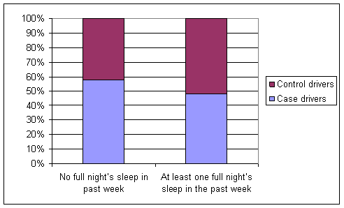
The odds of being involved in an accident are 1.48 times higher for those who did not get a full night’s sleep in the past week. The sample odds ratio is above one but not largely so.

(i) Example results:

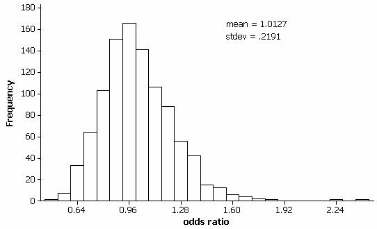
Description appears skewed to the right but the mean is close to the hypothesized value of 1.

(j) The above results have 27 of 1000 values as large or larger than 1.48, empirical p-value .027. This p-value would give moderate evidence to reject the null hypothesis and conclude that there is an association between the sleep variable and the accident variable.

(k) Example results:

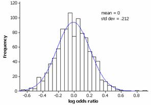
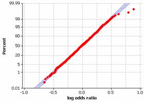
The distribution is approximately normal with mean approximately zero and standard deviation .212. We would predict a mean around zero since log(1) = 0.

(l) SE(log-odds) = sqrt(1/61 + 1/510 + 1/44 + 1/544) = .2072

This is similar to the value from the above simulation (.212).

(m) sample log odds = ln(1.48) = .392

.3920 + 1.645 (.2072) = .392 + .341 = (.051, .733)

We are 90% confident that the population log odds ratio is between .051 and .733.

(n) e^.051 and e^.733 gives a 90% confidence interval for the population odds ratio of (1.05, 2.08). We are 90% confident that the population odds ratio is between 1.05 and 2.08.

Investigation 5-4: Letrozole and Breast Cancer

(a) The women in this study were most likely volunteers and were not randomly selected from the populations of letrozole users and placebo users.

(b) This is an experiment since the women were randomly assigned to letrozole or placebo.

(c) H₀: d= 0 (no treatment effect)

H_a: d > 0 (the underlying rate of disease free survival is larger with letrozole than with placebo)

(d) Type I Error = we fail to detect that the letrozole therapy is helpful when we should

Type II Error = we believe that the letrozole therapy is helpful when really it is not.

(e) Yes, we have a randomized experiment and a two-way table.

(f) If we focus on the placebo group, we want to find P(X<2241)

Hypergeometric with N = 5157, M = 4631, and n = 2582

x P( X <= x )

2241 0.0000000

with such a small p-value, we reject the null hypothesis and conclude that the underlying rate of disease free survival is larger with letrozole than with placebo.

(g) Example results:

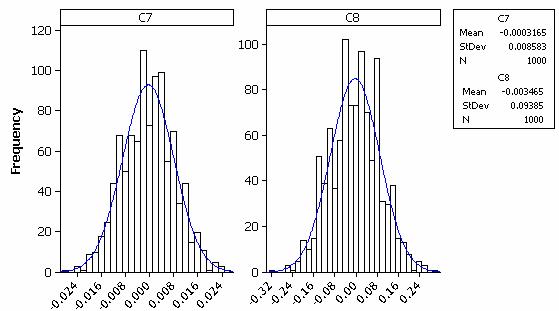
Both empirical randomization distributions appear to be reasonably well modeled by a normal distribution.

(h) Example results:

0/1000 = 0

(i) group X N Sample p

0 2390 2575 0.928155

1 2241 2582 0.867932

Difference = p (0) - p (1)

Estimate for difference: 0.0602235

95% CI for difference: (0.0437913, 0.0766557)

Test for difference = 0 (vs not = 0): Z = 7.18 P-Value = 0.000

Both p-values are essentially zero.

(j) exp(ln(1.966) + 2.576sqrt(1/2390 + 1/2241 + 1/185 + 1/341))

= exp(.676 + .247)

= (1.54, 2.52)

We are 99% confident that the underlying odds of disease free survival with letrozole are 1.54 to 2.52 times larger than the underlying odds of disease free survival with the placebo.

Investigation 5-5: NBA Salaries

(a) Obs units = NBA players

variable 1 = salary

“variable 2” = conference

These data constitute populations since they are for all players that season.

(b)

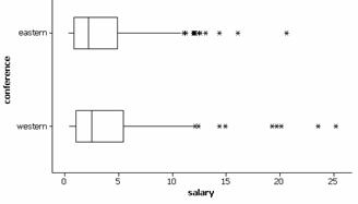
Variable conference N N* Mean StDev Minimum Q1 Median Q3

salary eastern 215 0 3.580 3.773 0.337 0.833 2.154 4.850

western 197 0 3.960 4.396 0.349 0.996 2.437 5.400

Variable conference Maximum Range IQR

salary eastern 20.630 20.292 4.017

western 25.200 24.851 4.404

Both distributions exhibit a slight skew to the right in the salaries. The distributions appear to have similar centers but the Western conference distribution has slightly more variability in the player salaries.

(c) Sample averages often follow normal distributions. The sample size is not large but the data are not extremely skewed either.

(d) Example results:

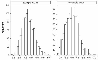
Variable N N* Mean StDev Minimum Q1 Median Q3

Esample mean 1000 0 3.6212 0.8146 1.4519 3.0229 3.5848 4.1499

Wsample mean 1000 0 3.9660 0.9057 1.9165 3.3034 3.9360 4.6016

Variable Maximum Range IQR

Esample mean 6.3541 4.9022 1.1270

Wsample mean 7.2960 5.3795 1.2982

Both distributions have a slight skew to the right. The centers are similar to the population means but the standard deviations are smaller.

(e)

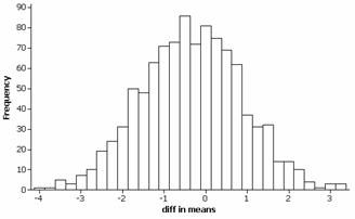
Variable N N* Mean StDev Minimum Q1 Median Q3

diff in means 1000 0 -0.3449 1.2072 -4.0075 -1.1656 -0.3370 0.4809

Variable Maximum Range IQR

diff in means 3.2271 7.2346 1.6465

The distribution of the differences in the sample means is symmetric with mean equal to the difference in the population means.

(f)

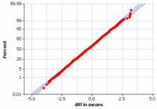
This distribution appears to be quite well modeled by a normal distribution.

(g) E( - ) = E() – E() by rules of expectation

= m₁ – m₂ (since and are unbiased estimators of m₁ and m₂)

(h) V( - ) = V() + V() by rules for variances with independent random variables

= s_x²/n_x + s_y²/n_y

SD( - ) = sqrt(s_x²/n_x + s_y²/n_y)

(i) 3.58 – 3.96 = -.38

sqrt(3.773²/20 + 4.396²/20) = 1.295

These should be pretty close to the simulated values.

(j) Possible suggestion

(k) t since that’s what happened before?

(l)

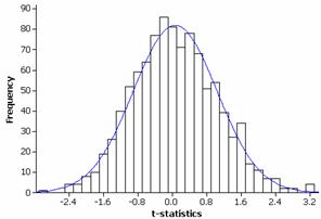
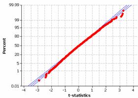
The distribution looks close to normal but again we see a little bit of heaviness in the tails suggesting that a t distribution might be the more appropriate model.

(m) Example results:

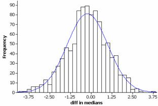
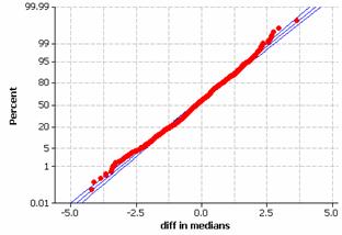
Investigation 5-6: Handedness and Life Expectancy

(a) This is a retrospective observational study. This implies that we will not be able to draw cause and effect conclusions from the results.

(b) These samples were not selected independently but membership in one group was not affected by membership in the other group so we will be willing to consider them as independent samples.

(c) This is crucial information for us to get a handle on the expected amount of sampling variability before we can decide if a difference of 75 vs. 66 is significant in a statistical sense.

(d) H₀: m_L = m_R (no difference in the mean lifetime of left-handers and right-handers)

H_a: m_L < m_R (the average lifetime of left-handers is smaller than that of right-handers)

(e) Calls for speculation.

(f)

Scenario		Sample sizes	Sample means	Sample SDs	t-statistic	p-value	Significant at 10% level?
1	left	99 (10% of 987)	66	15	-5.66	.000	Yes
	right	888	75	15
2	left	50 (5% of 987)	66	15	-4.13	.000	Yes
	right	937	75	15
3	left	50 (5% of 987)	66	25	-2.48	.008	Yes
	right	937	75	25
4	left	10 (1% of 987)	66	25	-1.13	.143	no
	right	977	75	25
5	left	99 (10% of 987)	66	50	-1.70	.046	Yes, but
	right	888	75	50

When the sample size for the left handers is larger, we have more evidence against the null hypothesis (larger t-statistics, smaller p-values). When the sample standard deviations are larger, we have less evidence against the null hypothesis.

(g) Probably scenario 1 or 2 as they have more a more realistic percentage of left-handers and the sample standard deviation is more reasonable (the others are too large if we are expecting about 35% of data values to fall more than one standard deviation above or below the mean – we probably aren’t expecting a normal distribution, but these standard deviations still feel too large).

(h) For even of the remotely realistic scenarios, the p-values were quite small indicating statistical significance.

(i) For scenario 1: 95% CI for difference: (-12.14685, -5.85315)

We are 95% confident that the average lifetime for right handers exceeds that of left handers by 5.8 to 12.1 years.

(j) For those who would be in their eighties in 1981, many of them would have been encouraged to not be left handed when they were younger. This would explain why there were fewer left-handers in the older age groups.

(k) Can’t impose whether or not someone is left handed.

Investigation 5-7: Comparison Shopping (cont.)

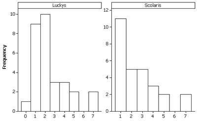
Variable N N* Mean StDev Minimum Q1 Median Q3 Maximum Range

Luckys 28 0 2.447 1.745 0.490 1.015 1.990 3.533 6.990 6.500

Scolaris 28 0 2.565 1.767 0.500 1.005 2.145 3.658 6.790 6.290

Variable IQR

Luckys 2.518

Scolaris 2.653

Both prices distributions are skewed to the right. There is a slight tendency for Scolari’s prices to be more expensive and the variability in the two distributions is similar.

(b) H₀: m_L = m_S (prices are the same on average – for all products common to both storess)

H_a: m_L < m_S (on average, prices are less at Lucky’s)

We are skeptical that the populations follow normal distributions but the shapes are similar and the sample sizes are close to 30 so we will proceed. The data were a random sample of products.

N Mean StDev SE Mean

Luckys 28 2.45 1.75 0.33

Scolaris 28 2.57 1.77 0.33

Difference = mu (Luckys) - mu (Scolaris)

Estimate for difference: -0.118214

95% upper bound for difference: 0.667631

T-Test of difference = 0 (vs <): T-Value = -0.25 P-Value = 0.401 DF = 53

With such a large p-value, we would fail to reject the null hypothesis. We do not have significant evidence of a lower average price at Lucky’s compared to Scolari’s.

(c) We don’t have two independent samples, one from each store, but instead we have one sample of products that was used at both stores.

(d) This controls for the variability in prices from product to product.

(e)

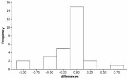
Variable N N* Mean StDev Minimum Q1 Median Q3

differences 28 0 -0.1182 0.3588 -1.0000 -0.2750 0.000000000 0.1000

Variable Maximum Range IQR

differences 0.7600 1.7600 0.3750

Most of the differences are around zero but the mean is slightly negative. The distribution of the differences is fairly symmetric.

(f) Let m = average price difference (Lucky’s – Scolari’s)

H₀: m = 0 (no price difference on average – for all the products common to both stores)

H_a: m < 0 (Lucky’s tends to have lower prices than Scolari’s, on average)

95% Upper

Variable N Mean StDev SE Mean Bound T P

differences 28 -0.118214 0.358774 0.067802 -0.002728 -1.74 0.046

With a p-value of .046, we have moderate evidence against the null hypothesis. At the 5% level of significance, we would conclude that the average price difference favors Lucky’s.

(i) The test statistic is larger and the p-value is smaller. The p-value has changed quite a bit.

(j)

	Lucky’s	Scolari’s	Difference
Mean	2.45	2.57	-.118
Standard deviation	1.75	1.77	.359

The variability in the differences is much smaller than the variability in the individual samples. This makes the difference in the sample means more “standard errors” from the hypothesized difference of zero.

(k) Variable N Mean StDev SE Mean 90% CI

differences 28 -0.118214 0.358774 0.067802 (-0.233701, -0.002728)

We are 90% confident that the average price savings at Lucky’s is between $.234 and $.003 per item. Comments on practical significance will vary for individuals. Would you be willing to pay more for gas to go to Lucky’s? Does it depend on how many items you tend to buy in one trip?

(l) Using Minitab:

Sign test of median = 0.00000 versus < 0.00000

N Below Equal Above P Median

differences 28 13 7 8 0.1917 0.00000

We would easily reject the null hypothesis and say we have statistically significant evidence that the median price difference is less than zero. More than half of the (differing) prices were lower at Lucky’s.

Investigation 5-8: Sleep Deprivation (cont.)

(a) H₀: d = 0 (no treatment effect)

H_a: d > 0 (lower improvement scores for sleep deprived group on average)

Two-sample T for improvement

sleep condition N Mean StDev SE Mean

deprived 11 3.9 12.2 3.7

unrestricted 10 19.8 14.7 4.7

Difference = mu (deprived) - mu (unrestricted)

Estimate for difference: -15.9200

95% upper bound for difference: -5.7644

T-Test of difference = 0 (vs <): T-Value = -2.71 P-Value = 0.007 DF = 19

Both use Pooled StDev = 13.4420

The p-value is quite similar to what we found before.

(b) 95% CI for difference: (-28.2128, -3.6272)

We are 95% confident that the true treatment effect from not getting that first night’s sleep is to lower the score by 3.63 to 28.21 on average.

(c) No, these were volunteer college students and may not be representative of a larger population.

Investigation 5-9: Heart Transplants and Survival

(a)

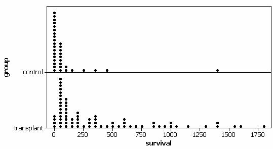
Variable group N N* Mean StDev Minimum Q1 Median Q3

survival control 34 0 96.6 250.3 1.00 5.75 21.0 54.8

transplant 69 0 415.3 458.6 5.00 70.0 207.0 645.0

Variable group Maximum Range IQR

survival control 1400.0 1399.0 49.0

transplant 1799.0 1794.0 575.0

Both distributions are strongly skewed to the right. The average survival appears much larger for the transplant group which also displays much more variability.

(b) It would be difficult to compare the means since there is “truncation” in the data, we don’t have the exact survival times for those still in the clinic.

(c) 207-21 = 186

(d) Example results:

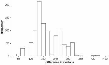
Variable N N* Mean StDev Minimum Q1 Median Q3

difference in me 1000 0 195.98 67.18 48.00 152.50 176.00 250.00

Variable Maximum Range IQR

difference in me 483.50 435.50 97.50

The distribution is irregular and skewed to the right with a mean around 195.95 and a standard deviation of 67.18.

(e) The standard deviation of the empirical bootstrap distribution of the differences in the group medians is: 67.18.

(f) The 25^th and the 975^th values.

(g) Example results: Sorting the observations, the 25^th value was 82 and the 975^th value was 322.

(h) This interval does not contain 0 but lies entirely above zero. This provides evidence of a statistically significant difference between the median survival time for those in the treatment group compared to the control group.

(i) If we instead looked at the 50^th and 950^th values, we get an interval of 95 – 316. This interval is less wide than the 95% bootstrap interval.

(j) Example results:

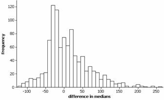
Variable N N* Mean StDev Minimum Q1 Median Q3

difference in me 1000 0 9.96 56.85 -121.00 -28.50 0.500 39.38

Variable Maximum Range IQR

difference in me 256.00 377.00 67.88

(k) 12/1000 or .012 is the empirical p-value for the above simulation.

(l) We have statistically significant evidence that the treatment effect is greater than zero, indicating a longer median survival time for those in the treatment group. This was an experiment so we can draw a cause and effect conclusion.

CHAPTER 6

Investigation 6-1: Dr. Spock’s Trial

(a)

	Judge 1	Judge 2	Judge 3	Judge 4	Judge 5	Judge 6	Judge 7
Proportion of women	.336	.270	.291	.341	.270	.270	.144

There is some variability in the proportion of women seen by each judge. Judge 7 in particular has a much lower percentage of women on his jury lists.

(b) Let p_i represent the probability of a female juror for judge i.

H₀: p₁ = p₂= p₃= p₄= p₅= p₆= p₇ (all seven judges have the sample probability of a female on the jury list)

H_a: at least one judge has a different probability

(c) The overall proportion of women in this data set is .261.

(d) Judge 1 saw 354 jurors so we would expect .261(354) = 92.39 females out of 354 and 261.61 men.

(e) Judge 2 saw 730 jurors so we would expect .261(730) = 190.53 women and 538.47 men.

(f) The expected counts are given below in red.

	Judge 1	Judge 2	Judge 3	Judge 4	Judge 5	Judge 6	Judge 7
Women on jury list	119 92.39	197 190.53	118 105.71	77 58.99	30 28.97	149 144.07	86 155.82
Men on jury list	235 261.61	533 538.47	287 299.30	149 167.01	81 82.03	403 407.93	511 441.18
Total	354	730	405	226	111	552	597

(g) The observed counts and the expected counts differ, however this could be due to random chance.

(h) Suggestions will vary.

(i) The sum is approximately 62.68

(j) This calculation will result in larger values when the null hypothesis is false and smaller values when the null hypothesis is true, but it will always be nonnegative.

(k) Example empirical sampling distribution (1000 observations):

This distribution is skewed to the right. The mean should be around 6.

(l) None of the simulated sums is anywhere near 62.68.

(m)

There is strong evidence that these observations do not follow a normal distribution.

(n) The distribution should seem reasonably well modeled by a gamma distribution with parameters approximately 3 and 2.

(o) This distribution also provides a reasonable fit.

(p)

To find the p-value we subtract this result from 1. This indicates a p-value of approximately zero.

The p-value from the chi-square distribution is near the p-value from the empirical sampling distribution.

(q) The contributions from Judge 7’s cells are the largest.

(r) The observed number of women is less than expected and the observed number of men is larger than expected. This provides evidence that the proportion of women for Judge 7 is less than expected, even more so than any of the other judges.

(s) Judge 7.

(t) C(7,2) = 21 comparisons

(u) P(Type I Error) = .05

(v) P(at least one Type I Error) = 1 – P(no Type I Errors) = 1- (.95)²¹ = .659.

Investigation 6-2: Near-Sightedness and Night Lights (cont.)

(a) hyperopia: .190, emmetropia: .524, myopia: .286

(b) There were 172 children in the darkness condition, so we expect 172(.19) and 172(.524) and 172(.286) or 32.68, 90.13, 49.19 in these 3 conditions.

(c) The proportional breakdown would be the same in all 3 groups if there was no association between eye condition and lighting level.

(d) Expected counts:

	Darkness	Night light	Room light	Total
Hyperopia	(40) 32.68	(39) 44.08	(12) 14.25	91
Emmetropia	(114) 90.13	(115) 121.57	(22) 39.30	251
Myopia	(18) 49.19	(78) 66.35	(41) 21.45	137
	172	232	75	479

(e) They are not the same but it could be due to random chance.

(f)

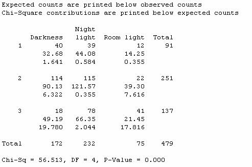
(g) The darkness/myopia cell and the room light/myopia cell have the largest contributions. We observed less myopia in the darkness group and more myopia in the room light group than we would have expected if there was no differences among the lighting groups.

Investigation 6-3: Newspaper Credibility Decline (cont.)

(a)

	2002	1998
4	200	265	465
3	391	353	744
2	251	235	486
1	90	69	159
	932	922

(b) H₀: The distributions of the believability ratings responses in the population were the same in 2002 and 1998.

H_a: There is at least one difference between the distributions.

The expected cell counts (see below) are all above 5 and we have independent random samples from 2002 and 1998.

We have strong evidence (p-value = .003) to reject the null hypothesis and conclude that the population distributions did differ.

(c) H₀: p₉₈ = p₀₂ vs. H_a: p₉₈ ≠ p₀₂

The expected cell counts are all above 5 (see below) and we have independent random samples from 1998 and 2002.

We fail to reject the null hypothesis. There is not convincing evidence that the population proportion who would rate their local paper as largely believable differed in 1998 and 2002.

(d) The test statistic we found before (z = -1.63) is smaller than the chi-squared value but the p-values are identical. In fact, squaring the z test statistic value gives the chi-square test statistic value.

Investigation 6-4: Handicap Discrimination

(a) The observational units are undergraduate students and the explanatory variable is the type of handicap, the response variable is the rating of candidate’s qualifications. This is an experiment since the undergraduate students were randomly assigned to view one of the types of handicaps.

(b) Sample size, sample standard deviation

(c) Let m_i = the true treatment effect for handicap type i

H₀: m_amp = m_crutch = m_hear = m_none = m_wheel

H_a: at least one of the m’s differs from the rest.

(d) Type I Error = thinking there is a difference in the effect of the handicap types when there is not.

Type II Error = thinking there is a not a difference in the effect of the handicap types when there is.

(e) The distributions appear similar in shape and center but have different amounts of variability within the groups. Graph B shows stronger evidence that the 5 samples did not all have the same overall mean.

(f)

There is some evidence of a difference in the average rating score given to the 5 different handicap types.

(g) The overall mean is 4.929.

(h) variance = .545

(i) Yes since the sample sizes are all equal.

(j) 14(.545) = 7.63

(k) average variance = (1.586² + 1.482² + 1.533² + 1.794² + 1.748²)/5 = 13.3357/5 = 2.67

(l) Our probability model is to consider the response ratings to be randomly assigned to the 5 treatment groups, so we expect similar variability in the 5 groups. This is confirmed by our observations from the numerical and graphical summaries of the results.

(m) 7.63/2.67 = 2.86

(n) Smallest value is zero which would result if there was no between group variation. There is no upper bound on the value this ratio can assume.

(o) This ratio will be large when the null hypothesis is false and small when it is true (but always nonnegative).

(p) We would put the 70 rating scores on index cards and then randomly assign 14 cards to 5 different groups and see what value of the test statistic we get for each randomization.

(q) Example empirical sampling distribution.

The empirical sampling distribution should be skewed to the right with mean about 1.

(r) Approximate p-value will be approximately .03 giving sufficient evidence to reject the null hypothesis at the 5% level.

(s)

(t)

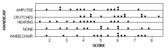
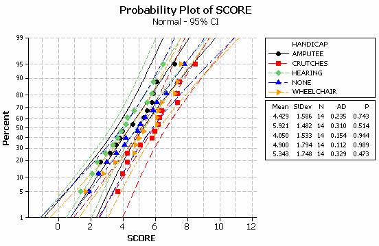
There is no evidence of nonnormality and the ratio of the largest to smallest sample standard deviation (1.794/1.482) is less than 2.

(u) There is moderate evidence that these average qualification ratings differ more than we would expect from the randomization process alone. There is at least one handicap that has a different effect on the qualification ratings than the other handicaps. The ANOVA procedure appears valid since the observed treatment group distributions look reasonably normal and treatment group standard deviations are also similar.

Investigation 6-5: Restaurant Spending and Music

(a) weighted average = [120(24.13) + 142(21.91) + 131(21.70)]/(120+142+131) = 22.52 (this is in the “middle” of the 3 observed averages).

Pooled variance = [119(2.243²)+141(2.627²)+130(3.332²)]/(119+141+130) = 7.73

Pooled std dev = sqrt(7.73) = 2.78 (this is in the “middle” of the observed standard deviations)

(b) H₀: the true treatment means (m_class = m_pop = m_none) are all equal

H_a: at least one true treatment mean differs

(c) variability between groups = 120(24.13-22.52)² + 142(21.91-22.52)² + 132(21.7-22.52)² /2 = 226

F = 226/7.73 = 29.2

F distribution with 2 DF in numerator and 390 DF in denominator

x P( X <= x )

29.3 1.00000

The p-value is approximately zero.

(d) We would need to be able to verify the technical conditions (in fact, there is an issue here in that the treatments were assigned to the evenings and not the individual dinners).

(e) Results will vary.

(f) Results will vary form sample to sample by chance.

(g) It will be possible to obtain a p-value below .05, but should happen less than 5% of the time (by chance alone).

(h) Now all the p-values should be quite small. We should have more evidence against the null hypothesis in this case since it is indeed false.

(i) The p-values tend to be larger, there will be less evidence against the null hypothesis from the smaller sample sizes (more variability due to chance).

(j) Larger values of s lead to larger p-values. This makes sense since larger values of s correspond to more variability in the treatment groups, making it harder to detect differences between the groups.

(k) The p-value will continue to get smaller since it will be easier to detect a difference when the size of the true difference is larger.

Investigation 6-6: House Prices

(a) The observational units are the 83 houses in the sample. The primary response variable of interest is the price of the house (quantitative)

(b)

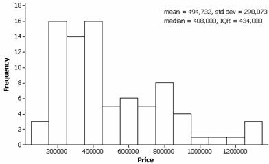
The distribution is skewed to the right with an average house price of around $494,732, a typical house price around $408,000 and an interquartile range of $434,000. The shape makes sense as there will be fewer of the more expensive homes.

(c) Best prediction for minimizing the sum of the square prediction errors would be the mean. The best prediction for minimizing the sum of the absolute prediction errors would be the median.

(d) Yes, there should be a tendency for larger homes to be more expensive.

(e)

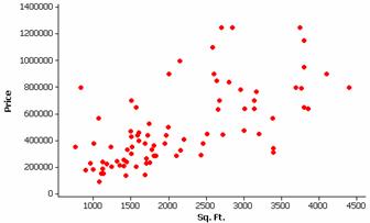
The pattern does seem to give evidence the size of the home is related to the cost of the house and in the expected way.

Investigation 6-7: Drive for Show, Putt for Dough

(a) Negative, golfers that hit further will tend to be the same golfers with lower scores.

(b) Positive, golfers that hit more putts will tend to be the same golfers with higher scores.

(c)

The relationship between average score and driving distance does appear to be negative. The relationship between average score and average putts appears positive and to be stronger than the first relationship.

(d) average score vs. average putts has more points in quadrants I and III

average score vs. driving has more points in quadrants II and IV

There appear to be fewer “unaligned points” in the average score vs. average putts graph.

(e) no measurement units

(f) the points will all fall exactly on a line

(g) 1

(h) no, involves means, standard deviations, and squared terms, all of which should contribute to it not being resistant to outliers.

(i) rankings may vary

(j)

Strong neg	Medium neg	Weak neg	No association	Weak pos	Medium pos	Strong pos
-.835	-.715	-.336	-.013	.356	.654	.884

(k) smallest in absolute value: 0, largest in absolute value: 1

(l) r will be negative when the association is negative and positive if the association is positive

(m) no association

(n) perfect linear relationship

(o) scoring average and average putts which does support the cliché that putting is more related to overall scoring.

Applet Exploration

(h) r = 1

(i) Not necessarily, you could just be consistently off by the same amount each time!

Investigation 6-8: Height and Foot Size

(a) The observational units are the students, the explanatory variable is the person’s foot length and the response variable is the person’s height.

(b) The mean height of the 20 students: 67.75

(c) No

(d)

74	66	77	67	56	65	64	70	62	67
6.25	-1.75	9.25	-.75	-11.75	-2.75	-3.75	2.25	-5.57	-.75
66	64	69	73	74	70	65	72	71	63
-1.75	-3.75	1.25	5.25	6.25	2.25	-2.75	4.25	3.25	-4.75

We overestimated 11 times and underestimated 9 times.

(e) The residual is positive if the observation is above the fitted value and negative if the observation is below the fitted value.

(f) Could consider sum of squared residuals, sum of absolute residuals.

(g) Positive, as expected, those with above average foot lengths are the same individuals with above average heights.

(h) Lines will vary.

(i) Predictions will vary.

(j) Points with positive residuals are above the line and points with negative residuals are below the line.

(k) No

(l) Suggestions will vary.

(m) SAE = 80.5, SSE = 475.8

(n) Lines will vary.

(o) Results will vary.

(p) The intercept is the predicted height for an individual whose foot length is zero.

The slope is the predicted change in height for foot lengths that differ by 1 cm.

(q) Could use calculus to find the values of the intercept and slope that minimize the sum of the squared residuals.

(r) derivative with respect to b₀: -2S(y_i- b₀ – b₁x_i)

derivative with respect to b₁: -2S(y_i- b₀ – b₁x_i)x_i

(s) Setting to zero:

Sy_i –b₁Sx_i = nb₀ b₀ = Sy_i/n –b₁Sx_i/n

Sx_iy_i –b₁Sx_i² = b₀Sx_i b₁ = [Sx_iy_i- b₀Sx_i]/Sx_i²

(t) b₁ = .711(5/3.45) = 1.03

b₀ = 67.75 – 1.03(28.5) = 38.4

predicted height = 38.4 + 1.03 footlength

Note: Will be lots of rounding discrepancies.

(u) SAE = 54.5, SSE = 235

These are smaller than when we use the line.

(v) predicted height = 38.4 + 1.03(28) = 67.24 in

This prediction will not necessarily have a smaller residual, but the overall sum of the squared residuals is as small as possible.

(w) predicted height = 38.4 + 1.03(44) = 83.72 in

The foot length of 44 cm is very far outside the range of the x values that were in the data set.

(x) 100%(475.8-235)/475.8 = 50.6%

Investigation 6-9: Money Making Movies

(a)

If we treat box office revenue as the response variable there is a moderate positive linear relationship between box office revenue and the critics score.

(b) The moves with the largest residuals include Lord of the Rings and Finding Nemo.

These movies had much higher box office revenues than we would have predicted based on the critics’ score.

(c) The correlation coefficient is r = .424 indicating a moderately strong, positive linear relationship.

(d) The regression equation is predicted box office = - 42.9 + 1.86 score

The intercept is the predicted revenue if the critics’ composite score is 0.

The slope is the predicted increase in box office revenues for a 1 point increase in the critics’ score.

(e) r² = 18% indicating that the regression on the critics score explains 18% of the variation in the box office revenues.

(f)

Most of the R movies are below the line. There are only a few G movies. The PG movies tend to be above or very close to the line. (Observations may vary a bit).

(g)

Most of the action movies appear above the line. Most of the dramas appear below the line. (Observations may vary a bit).

(h)

(i)

The relationship now appears much weaker (r = .299, only 8.9% of variation explained) but is still positive and linear. Those 6 movies had the effect of making the overall relationship look stronger.

Applet Exploration

(a) The relationship looks reasonably linear.

(c) This one point can dramatically change the slope, even making it negative.

(e) This point does not have as large an influence on the line.

(f) Points that are more extreme in the x direction appear to have more influence.

Investigation 6-10: Boys’ Heights

(a) Explanatory variable is age and the response variable is height.

(b) We expect there to be variability in the boys’ heights within ages but we also expect a tendency for the 3 year old boys to be taller than the 2 year old boys in general.

(c) It is possible that the sample slope differs from zero by chance.

(d) We could investigate what the lines look like when we choose random samples from a population where we know the population slope is equal to zero.

(e) population slope would be equal to zero.

(f)

The distributions look roughly normal with similar variability but different centers. The means each differ by about 6.

(g) These conditions do appear to be met for the Berkeley boys’ heights.

Investigation 6-11: Housing Prices (cont.)

(a) The regression equation is predicted price = 65930 + 202 square foot. r² = 42.1%

(b) Yes

(c)

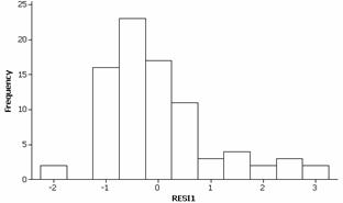
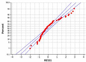
The residuals appear to be skewed to the right and not following a normal distribution.

(d)

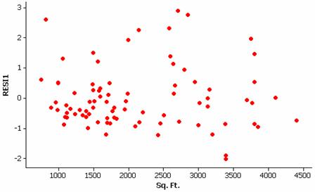
There does not appear to be strong curvature but the spread does appear to increase across the graph.

(e)

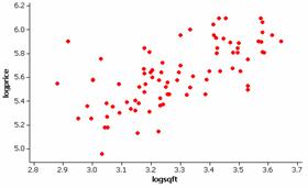
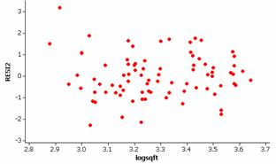
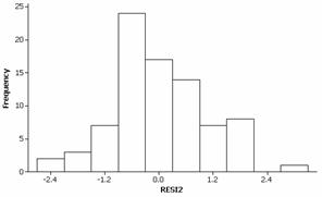
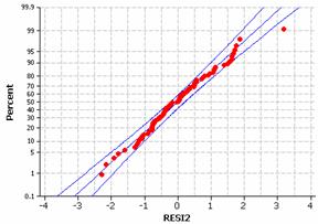
While not perfect, these variables do appear to better follow the basic regression model. The residuals appear less skewed and there is less variation in the “width” of the residuals at different values of the explanatory variable. There does not appear to be any curvature in the relationship either.

(f) The regression equation is predicted logprice = 2.70 + 0.890 logsqft. If the log square footage increases by one (which corresponds to a ten-fold increase in square footage), we predicted the log price will increase by .890 (which corresponds to a 10^.89-fold increase in price). If the log square footage is equal to 0 (square footage = 1), the predicted log price is 2.70 (price = 10^2.70).

(g) predicted logprice = 2.70 + .890 logten(3000) = 5.79

So the predicted price is 10^5.79 = $623,215.

Investigation 6-12: Hypothetical House Prices

(a) Yes it is possible.

(b) b₁ = 0

(c) H₀: b₁ = 0 indicating no relationship between the size and price of the homes in the population

H_a: b₁ ≠ 0 indicating there is a relationship between the size and price of the homes in the population.

(d)-(e) Regression lines will vary from sample to sample.

(f) The simulated regression lines “pivot” around the center of the graph.

(g) Shapes should be roughly symmetric. The mean of the sample intercepts should be around 5.62 and the mean of the sample slopes should be around 0. The standard deviation of the sample intercepts will be around .45-.50 and the standard deviation of the sample slopes will be around .15.

(h) The scatterplot is now not as wide in the vertical direction.

(i)-(j) There should be less swing in the lines vertically resulting in a smaller standard deviation for the sampling distribution of the sample slopes.

(k) There is less spread in the population in the horizontal direction.

(l)-(m) There will be more variability (larger standard deviation) in the regression lines from sample to sample.

(n)-(o) With a smaller sample size, there is more variability in the regression lines from sample to sample.

(p) Yes, n and s_X² are in the denominator and s is in the numerator.

(q) When there is less variation away from the regression line, there will be less variation in the sample regression lines, it is more difficult to get “extreme” regression lines. When there is less variability in the explanatory variable, we are not given as much information about the relationship between the two variables and it will be easier to get more extreme sample results. Larger samples, as always, lead to less sampling variability.

(r) .890 is a very extreme observation (doubtful anyone will ever observe a sample slope at least that extreme) and provides strong evidence that 0 is not a plausible value for the population slope.

(s) Now we may see one or two sample slopes as extreme as what the project group observed but .5 still does not appear to be a plausible value for b₁.

(t) Look at the residuals.

Investigation 6-13: Housing Prices (cont.)

(a) The variability about the regression line (estimate of s)

(b) t = 7.87 and p-value = .000/2 = .000

(c) If we were to repeatedly sample 83 houses from a population where there was no relationship between size and price, we would find a sample slope at least this extreme pretty much never.

(d) .196823*sqrt(1/(82*.192**2) = .1132

(e) t = .8899/.1131 = 7.87 Ö

(f) .8899 + ( t_n-2 )(.1131) = .8899 + (1.9897)(.1131) = (.665, 1.11)

We are 95% confident that the population slope is between .665 and 1.11 indicating that if we changed the log square footage by one, this is the range of the predicted change in the log price.

(g) The prediction at 2000 will be more precise because there is less variation in the location of the sample regression line for values of x closer to .

(h) No, 10,000 is too far outside the range of the explanatory variable values used to derive the least squares equation for this data set.

(i) Predicted Values for New Observations

New

Obs Fit SE Fit 95% CI 95% PI

1 5.6343 0.0217 (5.5911, 5.6774) (5.2403, 6.0282)

Values of Predictors for New Observations

New

Obs logsqft

1 3.30

width = 6.0282 – 5.2403 = .7879

(j) Predicted Values for New Observations

New

Obs Fit SE Fit 95% CI 95% PI

1 6.0596 0.0598 (5.9406, 6.1786) (5.6503, 6.4689)X

X denotes a point that is an outlier in the predictors.

Values of Predictors for New Observations

New

Obs logsqft

1 3.78

width = 6.4689 – 5.6503 = .8186

This interval is wider.

(k) The 95% CI reported by Minitab is (5.9406, 6.1786)

(see above output).

(l) This interval is narrower as it is “easier” to predict the average price of all homes at that size than to predict the cost of an individual house.

Minitab Exploration: The Regression Effect

(a)

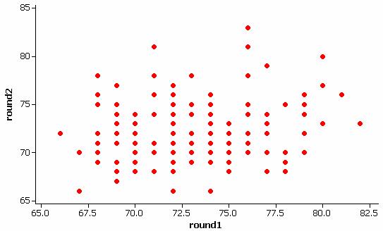
Based on the scatterplot and an r value of .140 we see a weak linear positive association between the round 1 and round 2 scores.

(b) Ten lowest:

Els, Ernie	66	72
Woods, Tiger	67	66
Flesch, Steve	67	70
Garcia, Sergio	68	69
Lehman, Tom	68	70
Paulson, Dennis	68	71
Harrington, Padraig	68	72
Garbutt, Ian	68	75
Maruyama, Shigeki	68	76
Dunlap, Scott	68	78

Ten highest

Ozaki, Naomichi	79	70
Little, Stuart	79	72
Da Silva, Adilson	79	74
Johnstone, Tony	79	75
Emerson, Gary	79	76
Karlsson, Robert	80	73
Trevino, Lee	80	77
Gillies, Colin	80	80
Fichardt, Darren	81	76
Jacobson, Fredrik	82	73

(c) Of the top ten golfers, only one improved in the second round. Of the bottom ten golfers, 9 improved and one tied his round 1 score.

(d) The bottom ten golfers were much more likely to see improvement.

(e) median of top ten golfers in second round: 71.5

median of bottom ten golfers in second round: 74.5

The top ten first round golfers were more likely to score better in the second round.

(f)

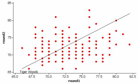
(g) The y=x line does not appear to do the best job summarizing the relationship in the scatterplot which appears to have a shallower slope.

(h)

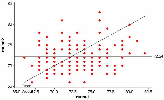
The line does not appear to do the best job summarizing the relationship in the scatterplot which appears to have a steeper slope.

(i)

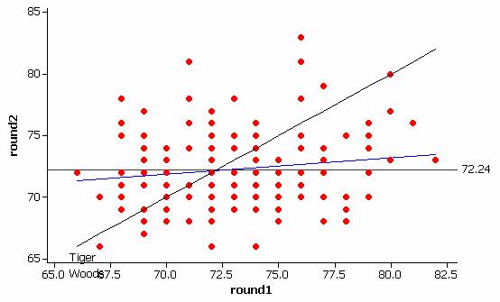
The regression line falls in between the two lines.

(j) predicted second round score = 62.43 + .1345 first round score

The slope is less than one.

The slope can be calculated through the equation b₁ = r s_y/s_x so when the standard deviations are similar, b₁ will be less than one since r must be less than (or equal to) one.

(k) Since the slope is less than one, golfers that have scores lower than average in the first round will tend to still be below average in the second round but not by as much (a change in 1 in x results in less than a 1 change in y). Golfers that have scores higher than average in the first round will tend to still be above average in the second round but not by as much.