INVESTIGATING STATISTICAL CONCEPTS, APPLICATIONS, AND METHODS, Third Edition
NOTES FOR INSTRUCTORS
August, 2024

Chapter 1       Chapter 2          Chapter 3     Chapter 4     Chapter 5

CHAPTER 3: COMPARING TWO PROPORTIONS

This chapter focuses on comparing two proportions but in a manner that mirrors the analysis process from Chapter 1. You can emphasize to students that the main structure is the same: determining good graphs and numbers to look at when analyzing the sample data, followed by inference procedures that build on an appropriate simulation model (but can lead to “exact” calculations and/or to large sample normal approximations) which allow us to make conclusions beyond the sample data. In fact, those conclusions will get more interesting as we get into issues of causation in addition to generalizability. The last section (Section 4) focuses on relative risk and odds ratios. These are skippable topics (or you can focus on descriptive but not inferential methods), though they also allow students the opportunity to apply the analysis process and thinking habits in new ways which can also be very empowering for students. These techniques will be very new to them but are much more representative of what they will see in the research literature. In fact, some statisticians argue the difference in conditional proportions is not a very useful statistic and should not be used. The distinction/comparison between standard deviations between random sampling and random assignment can also be skipped.

Section 1: Comparing Two Population Proportions

This first section extends what they saw in Chapter 1, comparing two population proportions arising from independent random samples, while raising new issues to consider with group comparisons (confounding). After Investigation 3.1, students turn to random assignment instead.

Investigation 3.1: Teen Hearing Loss (cont.)

Timing: If you have students use all of the new technology tools in class, including running their own simulations, this will take probably the first 50-min class period. Then the second class period can focus on applying the two-sample z-procedures, perhaps with an additional example. (There are two practice problems that can correspond to this split in days as well.)

Materials needed: If split over two days, you may want to have simulation results ready to discuss at the start of day 2.

You will want to enforce some caution in interpreting the difference in conditional proportions. Encourage students to always focus on the difference in proportions instead of percentages. As they will see if you discuss the material on relative risk, a “change of 10%” usually implies multiplication rather than addition/subtraction (vs. a 10 percentage point change). You will also want to caution students to be careful in describing how they conditioned their calculations (e.g., the proportion of senators who are male is very different from the population of males who are senators). You may also want to show Excel as an option for the segmented bar graph, and/or discussion mosaic plots.

For the simulation, to model the null hypothesis being true we assume the same value of  for each population. You can let students know that the particular value used for  in the simulation is not that critical, as long as it is the same for both populations. (A good follow-up question is why we didn’t use .15 and .19 as ₁ and ₂.) You will also want to make sure students are understanding the steps being performed by the simulation at each stage. Try to emphasize the common structure and the “why” behind the simulation steps. (Do watch for rounding issues in finding the p-value.) Questions (s) and (t) try to get them to think about how the standard deviation formulas are obtained and why we could make them differ for a test vs. a confidence interval. If you are short on time, you can emphasize the technology detour instead. Instructions for using a statistical package for the simulations rather than the applet are also provided but may not be as visual. Notice the simplification of the technical conditions made in the Summary box at the end of the investigation. When comparing proportions, students are often bothered about the direction of subtraction and how success and failure are defined, and you can have them work through some calculations to see how to make these adjustments from the first calculation.

Technology reminders: Using “+” when an R command continues onto the next line. They also have freedom to name vectors whatever they want. If you want to display multiple graphs, can use par(mfrow= c(r,c)), the first number is the number of rows and the second number is the number of columns, and then zoom the graph size as well. Also watch use of spacing with R commands so that you are not accidently replacing values. Column formulas can be a little annoying to work with in JMP. Try using the buttons as much as possible or you can always double click and edit directly (e.g., use a colon before column names).

Classic Sowell article

Investigation 3.2: Nightlights and Near-sightedness

Timing: A previous iteration of this activity as a class discussion, along with discussion of the practice problems, took approximately 30 minutes. (Students can be asked to work through 3.2-3.4 on their own in a 50-minute period with discussion the following class period.)

Materials: You may be able to find recent news articles related to this and/or similar studies.  Showing and critiquing these headlines in class can be motivating for students.

Students can first use these data to practice a two-sample z-test and confidence interval, but then this is a natural time to talk about drawing cause-and-effect conclusions. (This activity does discuss how you might conduct the simulation differently by modeling one random sample, classifying both variables, but we wouldn’t stress this at this point.) You can build on the teen hearing loss study, that even with a statistically significant difference between the two years, we aren’t able to isolate what might have caused the increase in hearing loss. Students are also usually pretty quick to develop (collaboratively) an alternative explanation in the night-light study. But you will want to make sure they are very clearly tying the alternative explanation (e.g., genetics) to both the explanatory variable and the response variable. The questions at the end of the investigation aim to help make the distinction between “other variables” and ones that are truly confounding variables with the explanatory and response in the study. Question (g) contrasts this with the issue of generalizability. The practice problems give them practice identifying and explanatory confounding variables and these are good ones to discuss in class as well.

Another very nice context here is the OK City Thunder home game record their second year in existence (see Exercise #4).  For similar data on the Sacramento Kings see this post.

Section 2: Types of Studies

So then we move into considering different study designs and how the scope of conclusions we can potentially draw differs based on the study design.

Investigation 3.3: Handwriting and SAT Scores

Timing: We have tried to streamline some discussion hear to address different study design and then explore the ability of random assignment to balance out groups in the same context.

This investigation begins with practice identifying explanatory and response variables as introduced in the previous investigation. In question (b), you will want to emphasize the self-selection of the subjects to conditions. Then two different study designs are compared. With experiments, we prefer to cite the imposition of the explanatory variable as the critical feature, with random assignment as the way to properly carry out such an experiment and only if you have both will you be able to draw cause-and-effect conclusions. The version of the Randomizing Subjects applet allows students to explore random assignment in this context with handedness. age, type of school, and amount of sleep as potential confounding variables. Students may not find the visualizations entirely convincing, so be sure to draw their attention to the goal of the random assignment process. We do make a big deal about the table at the end of this investigation and refer back to it many times in the course. We think giving them specific study contexts in each box can help them remember the distinctions as well.

Practice Problem 3.3 is probably the only one in the text that utilizes both random sampling and random assignment.

Investigation 3.4: Botox for Back Pain

Timing: Again can be used as class discussion (~30 min) or student exploration/practice. Some of the ideas will be new to students but you will want to emphasize that their common sense can be pretty useful here.

The main goals of this investigation are to expose students to a genuine excerpt from a journal article (show them how far they have come!) and to provide an opportunity to discuss more subtle issues with experimental design (e.g., standardized measurements, placebo treatments, realism/Hawthorne effect, and feasibility). Note “randomized” is mentioned in the title but not in the abstract. You may want to ask why the researchers didn't only examine the 11/15 statistic. The first practice problem provides additional practice identifying confounding variables, the provides additional practice with defining the key terms and their “statistical” meanings over the everyday meanings, and with the two components of scope of conclusions.  Practice Problem 3.4C emphasizes that even though they “did something” to the subjects, they did not impose the explanatory variable and therefore no causation can be drawn from the subjects’ emotions.

In general, students should also realize that experiments are not always feasible and/or can create an environment that is too artificial to be generalizable to the real world.

Here is a possible alternative version of the investigation. The only reason to switch would be to use a more current research study, the questions may not be as good (e.g., can’t have blinding in a study like this), but should still raise some important student design conditions (e.g., how measure hunger), repeated measurements on same individuals, random assignment, etc.  You might also want to find an article summarizing the study for comparison. For example, I found this article a little misleading compared to the actual student results. In particular, the results for ghrelin (the “hunger hormone”) are different than the hunger outcome.

Section 3: Comparing Two Treatment Probabilities

Now we return to investigating statistical significance, again starting with simulation, but now modelling the random assignment process rather than random sampling.

Investigation 3.5: Dolphin Therapy

Timing: The background material can take about 15 minutes and the card shuffling 10-15 minutes. Then using the applet and drawing conclusions can be another 15 minutes. If split over two days, getting through the tactile simulation on day one can work well.

Materials needed: For tactile simulation can use 30 playing or index cards, each pack with 13 of one type and 17 of another type (e.g., red vs. black, suits, face cards vs. non-face cards). More recently we have used colored index cards so students are less distracted by the type of card. Others don’t color code the cards but ask students to write “success” or “failure” on each card. The Dolphin Study applet link defaults to a version of the applet with the data pre-loaded in a 2x2 table. We feel the tactile simulation is still useful at this point in the course to help students see the distinction with random sampling.

Try to get them to think hard about question (d), even taking a few minutes to brainstorm in pairs.

After setting the stage, you will want to have some caution in defining the parameters as there are multiple approaches. One is in terms of treatment probabilities, but this may not feel very concrete (and different from the sample proportions) to students. Another is to define the parameters in terms of population proportions where you consider the populations to be all individuals who could potentially be on these treatments. You could also push students to consider the difference in probabilities as the one parameter of interest (vs. the individual probabilities as two parameters), to help them interpret confidence intervals later.

Depending on your class size, you may have enough repetitions even if each student (pair) repeats the process once or twice. In collecting the simulated data from the class, it is probably easiest to focus on the number of successes in group A rather than the equivalent difference in sample proportions. The latter calculation takes time (and more prone to error, but do make sure they all subtract in the same direction) and defining the random variable in terms of the count will be consistent with Fisher’s Exact Test when they turn to that. Still, you will want to emphasize to students the equivalence among the choices of statistics, and it is probably easier for them to think about why the difference in proportions in the null distribution should be near zero rather than thinking in terms of E(X). You can emphasize that the simulation is helping count how many “tables” are at least as extreme as the one observed.

In using the applet, the instructions don’t explicitly draw their attention, but you may want to, to the simulated bar graphs and how they vary when the null hypothesis is true vs. the observed results. If you check the Show Table box, you can edit the output in that window to copy (just the column titles and the table rows, not the total or prop rows) and paste into the Sample Data window. (Or just switch to the 2x2 table cell entry version.) You can also click on an outcome in the null distribution and the applet should display the corresponding shuffle (make sure you aren’t scrolled down in the page).

Some students may struggle with how this process fits into the earlier analyses (e.g., one sample or two random samples). You may want to use diagrams and/or concepts maps to help them see how this new ‘simulation structure’ fits into the larger picture. Also, in interpreting their p-value at this point, we try to emphasize whether they are talking about the percentage of random assignments vs. the percentage of random samples, and no longer letting them simply say “by chance.”

Investigation 3.6: Is Yawning Contagious?

Timing: 30-50 minutes (parts of this investigation can be assigned in advance)

Materials needed: Uses a generic two-way table inference applet. You can copy and paste the data (or URL) or enter own table (with spaces between columns and line breaks between rows, using just one-word row and column titles) and then press Use Table, or you can check the 2x2 box. You may be able to find a link to a video about this study at the Discovery website. Here is another video that’s a bit more focused on the study they will analyze. It’s also useful to emphasize how the research process is very iterative. Students can also be asked to view one of the videos between classes.

Students are given more practice and freedom in organizing the study results. Depending on the level of your students, you may want to go through several versions of the hypergeometric probability calculation by hand and even with the technology, practicing the appropriate input values depending on how the table is set up. (See also PP 3.6C.) Other students may ask about the conditioning on the observed data and there is actually some debate in the statistics community, but this is the standard approach (and hotly advocated by Fisher) especially for tables with smaller observed counts. Students will struggle with the distinction between binomial sampling (sampling with replacement) and hypergeometric sampling (sampling without replacement) and you will want think about how much to emphasize this.

Investigation 3.7: CPR vs. Chest Compressions

Timing: Investigation 3.7 focuses on descriptive statistics and the difference in proportions and the normal approximation. Investigation 3.8 focuses on relative risk and related inferential methods. The combination may take around 75 minutes.

This is another study that has been in the news and you may want to find recent articles and/or the current AHA recommendations. Students are given flexibility in setting up their table but this does impact the later components of the investigation so you may want to enforce some consistency (e.g., CC as the first column? Survival as the top row?) as you will return to this table frequently. This first investigation serves to apply the methods they have learned so far for comparing two proportions. Make sure students notice the direction implied in (d). Remind them in (h) that the 10% level really would have needed to have been set in advance.

The Practice Problem discusses follow-up analyses to this study but may not make the intended points as clearly, so make sure you discuss afterwards if used. You may want to emphasize to students that they are making predictions and then using technology to check their prediction (vs. being able to unambiguously know how the p-value will change in advance).

Section 4: Other Statistics

Investigation 3.8: Peanut Allergies

In this study, students begin to consider limitations to these calculations. In particular, when the probability of success is small to begin with, it can be difficult to interpret a small difference in conditional proportions. This motivates discussion of relative risk (and finally an interpretation in terms of percentage change). After establishing some benefits to examining relative risk, we next need to consider corresponding inferential methods for obtaining p-values and confidence intervals. So we go back to simulation. Here again we model the random assignment process rather than random sampling. This investigation relies on the two-way table applet to perform these simulations but code for R/Minitab/JMP macros can be found at the end of the investigation. Students should notice that the simulated randomization distribution is not the most normal/symmetric distribution. [The skewness is more prominent with smaller sample sizes. Here, some simulated tables will have zero successes. In this case, we add 0.5 to every cell in the table before calculating the relative risk.] But we can still find an empirical p-value. You will want to be especially careful with your rounding so that you don’t exclude the actual observed result from your tally. In fact, because of the one-to-one corresponding between the difference in conditional proportions and the relative risk, the “as extreme” outcomes are exactly the same ones as before and you should find the same empirical p-value.

But then how about confidence intervals – for that we need a standard error for this new statistic, but first we need to worry about the lack of symmetry. This motivates a transformation as they saw in Chapter 2. Students don’t seem to mind the standard error formula simply appearing. You apply the back transformation at the end and while the observed statistic will still be guaranteed to be in the interval, it is no longer necessarily the midpoint. Also make sure students realize why you want to consider whether the value one is in this interval rather than zero.

Technology notes: Keep in mind that R/Minitab/JMP assume natural log when you use “log” and that the standard deviation formula assumes natural log. When you look at the Minitab histograms, you may want to reduce the number of intervals to prevent strange binning and show a more “filled in” distribution. 

The Technology Detour for the simulation in R/Minitab pertains to a research study on a new flu vaccine (compared to the Hep A vaccination) (Jain et al., 2013).

	Hepatitis A vaccine	Quadrivalent influenza vaccine	Total
Developed Influenza A or B	148	62	210
Did not develop influenza	2436	2522	4958
Total	2584	2584	5168

 

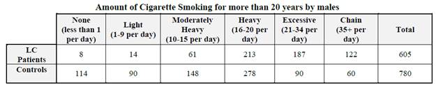
Investigation 3.9: Smoking and Lung Cancer 

Timing: 50 minutes 

This is a good historical example, building on three of the first major studies identifying a link between smoking and lung cancer. You can even find pictures of the original journal article title pages. If you discuss 2 or 3 of the studies, we encourage you/your students to ignore the slight differences in how the smoking variable is defined across the studies.

The investigation first distinguishes different types of observational studies. The key issue is we are not able to estimate the probability of lung cancer with a case-control study. This will be a difficult idea for students to get a handle on. The big consequence is that relative risk is not an appropriate statistic to examine, motivating discussion of odds ratio. You will want to go through these calculations very slowly and carefully with your students and continually emphasize that the interpretation now needs to be in terms of odds and not “chances” or “likelihood.” It is also fun to show students how much the relative risk can depend on how the two-way table is set up but the odds ratio is invariant. Some students will struggle with the relative risk and odds ratios calculations and interpretations, so try to give them plenty of practice. Once they have the odds ratio as an option for the statistic, we again give them a formula for the standard error and the transformation idea works as in the previous investigation - you may want to have students explore this outside of class. The visuals try to convey to students which results are held fixed and which are “random” (i.e., whether you are fixing the row or column totals to match the study design).

If you look at the full data table (different levels of smoking), the idea of “dose response” can be discussed but does not appear anywhere else in the text.

The second practice problem (and the later graphs) gives them more practice with odds ratio and seeing the distinction between relative risk and odds ratio.

Investigation 3.10: Sleepy Drivers

Timing: 25 minutes

This investigation is now just an opportunity to apply the odds ratio analysis outlined in the previous investigation. You might want to get students to think about how now the simulation should mimic the binomial sampling of the response variable categories based on the case-control design. Again, you will want to consider you much you want to emphasize this with students. Hopefully students are able to focus on the overall process by this point.

In this and/or the previous investigation, you may want them to explore how the standard error will differ for random sampling vs. random assignment and whether or not you assume the null hypothesis to be true (similar to using a pooled estimate of  or not with confidence intervals for the difference in population proportions in Chapter 3).

End of Chapter

Again, make sure students notice the examples and the end of chapter reference material. The software quick reference guides have been readded at the end.

Example 3.2 is a new context (Fall 2023) that has potential for even more analysis. For now, we have focused on how the size of the difference between proportions and the sample sizes impact the p-value. You can also revisit the discussion of statistical vs. practical significance and how the ratio of proportions may be a more meaningful comparison than the difference. A better introduction could be this statement from a recent NY Times article:

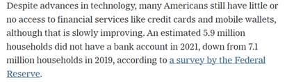
There are also numerous resources at that website, including the code book and discussion of how this is a supplemental survey to the CPS. The materials also discuss imputation and weighting of responses. You can also have students easily create their own data tables for other comparisons of their choosing. The link in the example gives only the race and income variables but you can also download the full raw dataset.