BRIEF SOLUTIONS TO INCLASS INVESTIGATIONS – Chapter 2
Last Updated November
5, 2013
Investigation 2.1:
Teen Hearing Loss (cont.)
(a) difference: compare 2 groups
same: binary, categorical variable
(b) populations: 1. 2005-6 teens; 2. 88-94 teen
Variable: whether/not some hearing loss. Binary categorical
(c)
|
|
1988-1994 |
2005-2006 |
Total |
|
some hearing loss |
480 |
333 |
813 |
|
no hearing loss |
2448 |
1438 |
3886 |
|
Total |
2928 |
1771 |
4699 |
(d) Because the sample sizes for the two surveys are not the same
(e) ![]() 88 –
88 – ![]() 05 = 480/2928 – 333/1771 = -0.024
05 = 480/2928 – 333/1771 = -0.024
(f)
A slightly higher proportion of teens (.024) had some level of hearing loss in the 2005/6 data than in the first data set.
(g) yes! Random sampling “error”
(h) H0: ![]() 94 –
94 –![]() 06 = 0 (the
population proportions are the same)
06 = 0 (the
population proportions are the same)
Ha: ![]() 94 –
94 –![]() 06 < 0 (a
higher rate of hearing loss in 2006 than in 1994)
06 < 0 (a
higher rate of hearing loss in 2006 than in 1994)
Success = some hearing loss
(i) how
often ![]() 1
–
1
– ![]() 2
£
-0.024 when
2
£
-0.024 when ![]() 94 –
94 –![]() 06 = 0 by
random sampling alone.
06 = 0 by
random sampling alone.
(j) random sampling when![]() 94 =
94 = ![]() 06 =
06 = ![]()
(k) 813/4699 = 0.173
(l) Assume the population proportion is 0.173. Take independent random samples from this population, one with 2928 observations and one with 1771 observations. Determine the difference in the sample proportions. Repeat this a very large number of times to create the “what if” distribution. Count how many of these “could have been” statistics are -0.024 or smaller. That’s the p-value.
(m) usually less extreme – expect difference to be 0
(n) no, because of the randomness in the sampling process
(p) No question
(q) The distributions of the ![]() values should be approximately normal with
means around 0.173. The standard deviations should be around .007 and
.009. The distribution of the
values should be approximately normal with
means around 0.173. The standard deviations should be around .007 and
.009. The distribution of the ![]() 1-
1-![]() 2
values should be approximately normal with mean around 0 (.173 – .173) and
standard deviation around 0.11.
2
values should be approximately normal with mean around 0 (.173 – .173) and
standard deviation around 0.11.
(r) about 0.017
This is a small p-value and provides moderate evidence against the null hypothesis in favor of the alternative hypothesis that the population proportion with at least some level of hearing loss was greater in 2006 than in 1994.
(s) The normal distribution
(t) Yes
(u) Larger. This makes sense because we now have two sources of variability and the overall amount of variation will grow. (For example, we could get two extreme results, in opposite directions, and end up with a large difference.)
(v) = z
= z
(w) ![]() 94
–
94
– ![]() 06
= -0.024
06
= -0.024
![]() = 0.173
= 0.173
SE(![]() 94
–
94
– ![]() 06)
=
06)
=![]() = .0113
= .0113
Test statistic: z=![]()
Interpretation: Our ![]() 1
–
1
– ![]() 2
(-0.024) is 2.12 standard errors below the mean (
2
(-0.024) is 2.12 standard errors below the mean (![]() 1-
1-![]() 2=0)
2=0)
(x) yes
(y) P(Z < -2.12) ≈ .017
(z) estimate ± (critical value)(standard error)
![]() 1 –
1 –![]() 2 ± z*
2 ± z* ![]()
(aa)
-0.024 ± 1.96![]() = (-0.047, -0.001)
= (-0.047, -0.001)
We are 95% confident that the population proportion of at least some hearing loss in 2006 is .001 to .047 larger than the population proportion with at least some hearing loss in 1994. This interval is consistent with our test because all of the values are negative (we rejected zero as a plausible value for the difference in population proportions in favor of the alternative that the probability of hearing loss was now larger). Technically we should adjust this comparison for the one-sided nature of the significance test. For example, the two-sided p-value would be .034, so we expect zero to not be included in the confidence interval for any confidence level of 96.6% or less.
(bb) The change in the likelihood of some hearing loss in these two samples is statistically significant (p-value = 0.017 from z-test) and we are 95% confident that the population proportion is 0.001 to 0.047 higher “now” than before among all American teenagers (representative samples by NHANES).
NOTE: The adjective “statistically significant” applies to the sample data, not the population data.
Investigation 2.2:
Nightlights and Near-Sightedness
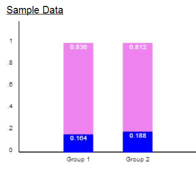
(a) ![]() with light: 188/307 =
.6124
with light: 188/307 =
.6124
![]() without light: 18/172
= .1047
without light: 18/172
= .1047

There appears to be a large increase in the proportion of near-sightedness between children who used light in the room vs. children who did not (51 percentage points). The difference appears large and is likely to be statistically significant.
(b) We could construct a population where 206/479 or about 43% are near-sighted and 307/479 or about 64% use light in the room. Then we could randomly select a sample of 479 children from this large population and classify the selected children according to both variables and then see how often we get a difference in conditional proportions at least as large as the observed. (Note, this would allow both sets of marginal totals to vary from sample to sample.)
(c) H0: ![]() light –
light – ![]() dark = 0 (no
difference in the population proportions)
dark = 0 (no
difference in the population proportions)
Ha: ![]() light –
light – ![]() dark
dark![]() 0 (there is a difference in the population
proportions)
0 (there is a difference in the population
proportions)
Two-sample z-procedures:
![]()
We have very strong evidence (p-value < .001) to reject the null hypothesis. We conclude that the probability of myopia is .436 to .579 larger for those who sleep with a room light above those children who sleep in darkness.
(d) No, a small p-value only convinces us that the results did not occur “by chance alone.”
Several possible explanations. One is that children inherit near-sightedness from parents and maybe near-sighted parents use more light to see.
(e) If birth weight impacts eye condition and birth weight differs across the 2 lighting groups
(f) Not if didn’t differ across the 2 lighting groups. Clinic was the same for the two groups.
Investigation 2.3:
Handwriting and SAT Scores
(a) Explanatory variable: cursive or block letters (writing style)
Response variable: SAT score
(b) No, there are lots of potential confounding variables, such as the students’ educational background. Maybe students from private schools are more likely to use cursive and more likely to have taken SAT prep courses to score highly on the exam.
(c) Now there are no differences between the essays other than the writing style.
(d) Yes, the writing style should be the only explanation for a difference between the scores.
(e) Use of 2006 exams: observational
Use of one version written both ways: experimental
(f) The essays are identical except for the writing style
(g) This is less realistic as the judges are in an artificial situation rather than truly scoring the exam in a natural setting.
Investigation 2.4:
Have a Nice Trip
(a) No, then gender would be confounding with treatment. Need to use random assignment and imposition of explanatory variable.
(b) We’d expect 8 of the 16 males in the elevating group to be male and 8 of the 16 females in the lowering group to be male. But this certainly wouldn’t happen every time, there could be “random errors.”
(c) Results will vary.
(d) Results will vary but it’s quite probable the difference will change.
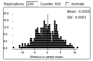
(e) Example results:
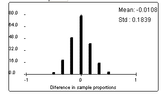
The pattern is very symmetric with a peak at 0.
(f) Not always, but there is certainly a tendency to create groups with equal or almost equal proportions of males.
(g)
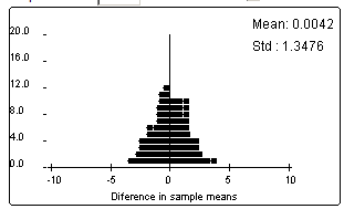
Yes, the center of this distribution is also zero.
(h)
Yes, the center of this distribution is also zero.
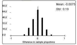
(i) Yes, the center of this distribution is also zero.
(j) We would draw a cause-and-effect conclusion between the strategy and the ability to recover because this was a randomized, comparative experiment. We aren’t sure how they selected the subjects though, so we would be cautious in generalizing these results to a larger population.
Investigation 2.5:
Botox for Back Pain
(a) This is an experiment because the researchers determined which patients would the botox and which the saline.
(b) To guard against other things changing during the same time period (e.g., back pain just going away over time). We need that to be the same in both groups so that we can further isolate the effects of the botox.
(c) So that participants won’t know which treatment they are receiving.
(d) This will equalize any psychological effects from receiving a treatment that you are told will help you feel better.
(e) Random assignment; to create equivalent groups
(f) To ensure the response variable is measured consistently and without bias (so person taking the measurements also should not know which treatment the patient received).
(g) To help inform as to which population we are willing to generalize the results.
(h) Probably not feasible to impose the lighting condition on the children.
Investigation 2.6:
Dolphin Therapy
(a) obs units: depressed people
variable 1: experienced substantial or not (response variable)
variable 2: did you swim with dolphins (explanatory variable)
(b) This is an experiment because the researchers determined whether or not each person would swim with dolphins.
(c) ![]() d –
d – ![]() c
= 10/15 – 3/15 = 7/15 = 0.467
c
= 10/15 – 3/15 = 7/15 = 0.467
(d) The data are in the direction of a higher chance of substantial improvement if swim with dolphins.
(e)
Ho: ![]() dolphin –
dolphin –![]() control = 0
(no difference in the treatment probabilities)
control = 0
(no difference in the treatment probabilities)
Ha: ![]() dolphin –
dolphin –![]() control >
0 (those in dolphin treatment are more likely to show substantial improvement)
control >
0 (those in dolphin treatment are more likely to show substantial improvement)
(f) The null model is that there is no difference between the two groups. So we want to simulate using random assignment to separate 30 people into 2 groups of 15, where was assume there are going to be 13 improvers and 17 non-improvers no matter which group they end up in. See how often we get a difference in the conditional proportions of .467 or larger.
(g) results will vary
(h) results will vary, but notice that the row and column totals do not change
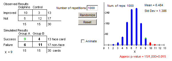
(i) Example results
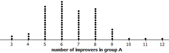
(j) observational units are the shuffles (or random assignments) and variable is the number of improvers (successes) in group A (dolphin therapy)
(k) Getting 10 or more of the 14 successes in group A looks pretty unusual
(l) results will vary
(m) Yes, the number of successes varies from repetition to repetition
(n) 10, yes
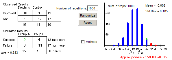
(o) about .015
(p) 6.5, about half the improvers should end up in the dolphin group
(q) The scaling changes and the mean is now zero, the p-value does not change
(r) The simulation helps us see the distribution of results we are likely to get when we know for sure the null hypothesis is true and any differences that do arise between the two groups is strictly from the random assignment process. Because we obtained a difference between the groups that is larger than most of those produced by the random assignment process under the null, we have strong evidence that our results aren’t just from an unlucky random assignment and instead reflect a genuine treatment effect.
(s) We might be willing to attribute this difference to dolphin therapy alone as they tried very hard to have identical conditions for the two groups apart from the dolphins (more on this later)
(t) We might be willing to generalize this is depressed people with similar symptoms, ages, geographical region etc., but should be cautious as these folks were recruited through newspaper, radio, and online advertisements and might not represent this larger population.
Investigation 2.7: Is
Yawning Contagious?
(a) EV: given seed or not
RV: whether yawned or not
(b) Parameter: ![]() s –
s –![]() c =
difference in probability of yawning (seeded – control)
c =
difference in probability of yawning (seeded – control)
H0: ![]() s –
s –![]() c = 0 (no
association between seeding & yawning)
c = 0 (no
association between seeding & yawning)
Ha :![]() s –
s –![]() c > 0 (the yawn seed leads to a higher probability
of yawning)
c > 0 (the yawn seed leads to a higher probability
of yawning)
(c) unequal sample sizes so need proportions
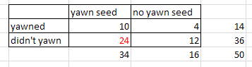
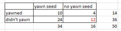
(d)
|
|
seed |
no
seed |
total |
|
yawn |
10 |
4 |
14 |
|
no
yawn |
24 |
12 |
36 |
|
|
34 |
16 |
50 |
(e) 50 cards. 14 red, 36 blue. Shuffle. Deal out 34 to “group A”.
(f) symmetric (but with gaps
depending on rounding/bins), mean(![]() 1
–
1
– ![]() 2)
≈ 0, sd(
2)
≈ 0, sd(![]() 1
–
1
– ![]() 2)
≈ 0.14
2)
≈ 0.14
(g) p-value about 0.5
(h)![]() = possible ways to randomly assign 34 people
to group A.
= possible ways to randomly assign 34 people
to group A.
(i) Successes:![]()
Failures:![]()
(j) X = # successes in group A
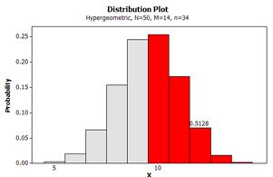
P(X = 10) =![]() = 0.254
= 0.254
(k) no, need P(X ≥ 10) not P(X = 10)
(l) P(X=11) » .1708, P(X=12) » .0702, P(X=13) » .0158, P(X=14) » .0015
stop at 14 because total # successes
(m) exact p-value = 0.5128
comparison: similar to simulation
interpretation: P(X ≥ 10), probability of 10 or more successes by random assignment alone (assuming no effect from the seed).
(n) P(X > 10) with M = 14, n = 35, N = 50
(o) P(X < 24) with M = 36, n = 35, N = 50 = 0.5128
(p) P(X > 12) with M = 36, n = 16, N = 50 = 0.5128
(q) The simulation results should be very similar.
(r) The p-value is not small so we fail to reject H0, not convincing evidence of a seeding effect
(s) No! We are not able to discount “chance” (random assignment) as the explanation for the observed difference in the sample proportions.
Investigation 2.8:
CPR vs. Chest Compressions
(a) Observational units = 518 cases
Explanatory variable = whether they were given CPR or CC instructions
Response variable = whether the patient survived to discharge from the hospital
Type of Study = experimental
(b) There are many appropriate ways for constructing a two-way table, with the explanatory variable as the column. Below is one example.
|
|
CPR |
CC |
Total |
|
Survive |
29 |
35 |
64 |
|
didn’t survive |
249 |
205 |
454 |
|
Total |
278 |
240 |
518 |
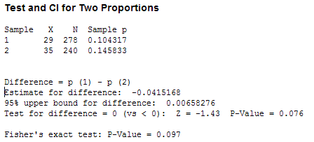
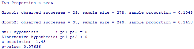
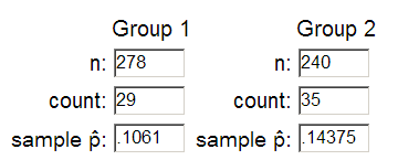
(c) ![]() cc -
cc - ![]() cpr = 35/240 - 29/278 = .0415
cpr = 35/240 - 29/278 = .0415
Opinions will vary on whether this difference appears noteworthy.
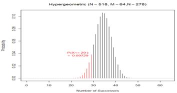
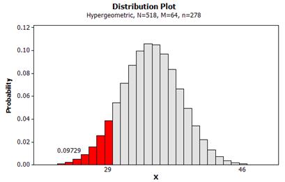
(d) Let X count the number of survivors in the CPR group. Note, we are “assessing the strength of evidence that the probability of survival is higher with CC alone.”
exact p-value = P(X < 29 with M = 64, n = 278, N = 518) = .0973
![]()
|
|
|
(e) The p-value is a little smaller.
|
|
|
|
|
|
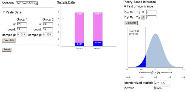
(f) continuity correction
(g) To make sure the probability mass at 29 is included, we could consider finding the probability for something just above 29 (e.g., 29.5).
|
|
|
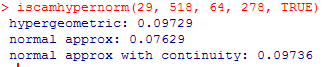
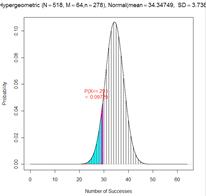
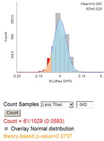
The p-value from the normal distribution is a little low but the continuity correction makes the approximation much more accurate.
Note, in the TOS applet, we can use 29.5/278 = .1061 and 34.5/240 =.14375 to achieve this effect
|
|
|
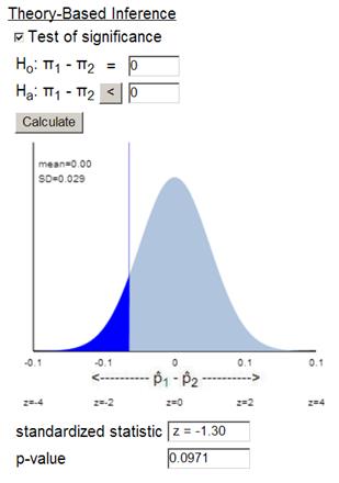
(h) Yes, the exact p-value of .09736 is below .10, so we would consider this convincing evidence at the 10% level.
(i) 90% CI for ![]() cpr –
cpr – ![]() CC: (-.0896,
.0066)
CC: (-.0896,
.0066)
I’m 90% confident that the survival probabilities is up to .0896 higher for the CC group but could be up to .0066 higher for the CPR group.
(j) The observed statistic would now be positive 0.042
The test statistic would now be positive (but same magnitude)
The p-value, now the probability of a statistic above 0.042, would be the same.
(j) It’s a little dissatisfying that zero is inside the interval when we rejected zero as a plausible value in (h), but that was using a one-sided alternative. The other issue is even .0896 is not all that large of a value, so it’s not clear whether the CC treatment has a “large” benefit.
Investigation
2.9: CPR vs. Chest Compressions (cont.)
(a) The difference is small because the proportions used in the difference are small. Whereas when the proportions are closer to .5, the same difference doesn’t seem as large.
(b) Relative risk (CC/CPR) = (35/240)/(29/278) = 1.398
Those getting CC were 1.398 times more likely to survive that those getting CPR,
(c) Those getting CC were 40% more likely to survive that those getting CPR.
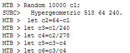
4. phatCC = CCsurvive/250
phatCPR = CPRsurvive/278
diff = phatCC – phatCPR
ratio = phatCC/phatCPR
|
R > CCsurvive=rhyper(10000, 64,
454, 240) > CPRsurvive=64-CCsurvive > phatCC = CCsurvive/240 > phatCPR = CPRsurvive/278 > diff=phatCC-phatCPR > ratio=phatCC/phatCPR |
Minitab |
(d) The values in CCsurvive represent the randomly generated number of survivors in the CC group after the 64 survivors (and nonsurvivors) were randomly shuffled and dealt to two groups.
(e) Example results
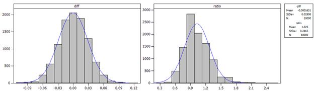
As expected, the distribution of the differences in the conditional proportions is well-modeled by a normal distribution. However, the distribution of the relative risks is not as well-modeled by a normal distribution (with mean 0). In fact, the distribution appears to have a shorter left tail and a longer right tail (aka “skewed to the right”).
(f) The mean of the ratios is about 1. This makes sense because under the null hypothesis, the conditional probabilities are the same and so the ratio will equal one.
(g) 1.397 is a little bit out in the tail of the distribution of the ratios, but not extremely so.
|
R >
sum(ratio>=1.397)/10000 |
Minitab MTB > let
c7=(c6>=1.397) MTB > let
c8=sum(c7)/10000 |
Results will vary from student to student, but the p-value should be close to .097.
(h) the approximate p-value should be the same (if using the same simulated values)
(i) Yes, example results below
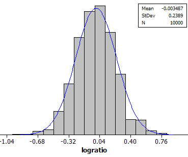
(j) about zero (because log(1) = 0)
(k) about 0.24
(l)![]() = .235
= .235
This tells us how much sample to sample variation there is in the log-relative risk values and is similar to what was found in the simulation.
(m) log(1.389) + 1.96 (.235) Þ (-.126, .796)
(n) log(![]() 1/
1/![]() 2)
2)
(o) (e-0.126, e0.796) = (0.882, 2.22)
I’m 95% confident that the “true” relative risk (![]() 1/
1/![]() 2) is in here,
meaning the probability of survival with CC is up to 2.22 times (122%) higher
than with CPR or 12% lower.
2) is in here,
meaning the probability of survival with CC is up to 2.22 times (122%) higher
than with CPR or 12% lower.
(p) value of interest: 1
(q) 1.398, this is not the midpoint but makes sense because the distribution of ratios was not symmetric.
(r) If the simulations are done under the null hypothesis, so that 1 is the actual value of the parameter, then in the long run we would expect 95% of these 95% confidence intervals to include the value one. Every once in a while (5% of the time) we will generate samples that fail to capture the true parameter value.
Investigation 2.10:
Smoking and Lung Cancer
(a) EV = whether or not male was a regular smoker
RV = whether or not the male had lung cancer/died of lung cancer
(b) Wynder and Graham: Observational
Hammond and Horn: Observational
In neither study did the researchers impose the smoking status
(c) W&G: found people with lung cancer or not, asked about smoking habits
H&H: found smokers/non-smokers, watched for lung cancer
Night light: found children and asked about light use and checked vision.
(d)
|
|
Wynder and Graham |
Hammond and Horn |
|
Advantages |
-
gather data at once -
ensure a large number of cases/controls |
-
easier to continue to get data |
|
Disadvantages |
-
still observational -
recall bias -
can’t estimate the “risk” of lung cancer |
-
what other factors happen
over time? -
time consuming -
not sure how trained/consistent the interviewers are |
(e) Night lights: cross-classified
W&G: case-control
H&H: cohort
(f) W&G RR![]() =
=![]() = 5.17
= 5.17
H&H RR![]() =
=![]() = 10.73
= 10.73
The Hammond and Horn, with the larger relative risk, shows a stronger connection between smoking habits and lung cancer.
(g) No, these are observational studies so no cause-and-effect conclusions can be drawn. Possible confounding variables include genetics or overall lifestyle (e.g., those who smoke may also have more poorer diets and get less exercise)
(h) No, it would not be appropriate to use these data to estimate how often males are hospitalized with lung cancer because the researchers chose how many to sample from each group rather than observing the natural breakdown.
(i) This is ok but might have to adjust for % of smokers/non-smokers.
(j) If the distribution of a variable is controlled by the researcher it is not appropriate to make inferences about the outcomes of that variable in the population. In the W&G study, the researchers manipulated how many lung cancer/control patients they had, but in the H&H study, the lung cancer variable was recorded “naturally.”
(k) RR of smoking = LC/control =![]() = 1.305
= 1.305
The risk of smoking was 1.305 times higher for lung cancer patients then for control patients.
This is a valid calculation because the variable we are looking at (smoking status) was not controlled by the researchers.
However, this value is quite a bit smaller than what we say in (f) and does not indicate nearly as strong of a relationship between the two variables.
(l) non-regular: 22/204 = 0.108 -- so roughly 1 to 10 odds of having lung cancer (10 times more likely to not have lung cancer than to have lung cancer)
regular: 583/576 = 1.012 – so roughly 1 to 1 odds of lung cancer (equally likely to have lung cancer not)
The regular smokers have higher odds of lung cancer.
(m) OR = 1.012/0.108 = 9.37
The odds of lung cancer are about 10 times greater for regular smokers compared to non-smokers (going from .1 to 1.).
The relative risk was 5.17, not all that similar.
(n) OR =![]() = 9.39 (same)
= 9.39 (same)
RR = 1.305
(o) The odds ratio calculations don’t change, but the relative risk calculations do.
|
|
odds ratio |
relative risk |
|
of lung cancer comparing smokers to
non-smokers |
(583/576)/(22/204) = 9.385 |
|
|
of not having lung cancer comparing
non-smokers to smokers |
(204/22)/(576/583) = 9.385 |
204/226/(576/1159) = 1.816 |
|
of not having lung cancer comparing smokers
to non-smokers |
(576/583)/(204/22) = .1065 (=1/9.385) |
576/1159/(204/226) = .551 |
|
of lung cancer comparing non-smokers to
smokers |
(22/204)/(583/576) = .1065 |
(22/226)/(583/1159) = .194 |
|
of being a smoker comparing lung cancer
patients to controls |
(583/22)/(576/204) = 9.385 |
|
(p)
|
Light vs. none |
mod heavy vs none |
heavy vs none |
excessive vs none |
chain vs none |
|
|
4.88 |
10.92 |
29.6 |
29.0 |
(q) odds ratio increases the more you smoke (this indicates that the more you smoke the higher the chances of lung cancer)
Investigation 2.11:
Sleepy Drivers
(a) The observational units are drivers; Explanatory variable is whether or not got a full night’s sleep in previous week; Response variable is whether or not were involved in a car crash; This is a case-control observational study.
(b)
|
|
No full night’s sleep |
Full night’s sleep |
Total |
|
Crash |
61 |
535-61 = 474 |
535 |
|
No Crash |
44 |
588 – 44 = 544 |
588 |
|
Total |
105 |
1018 |
1123 |
(c) If we look at the odds of being in a crash if they did not get a full night’s sleep compared to the odds of being in a crash if they did get a full night’s sleep: (61/44)/(474/544) = 1.5911
Note, this is the same as the odds of not getting a full night’s sleep for the crash victims vs. the odds of not getting a full night’s sleep for the non-crash subjects.
The odds of being in a crash if didn’t get a full night’s sleep were 1.59 times higher than the odds of being in a crash if did get at least one full night’s sleep.
(d) The p-value, specifically how unusual it is to get an sample odds ratio as extreme as 1.59 if there really is no association between these two variables in the population.
(e) H0: t = 1 (the population odds ratio is one, there is no association between sleep and crash)
Ha: t > 1 (note, it’s not clear here whether they had a one or two sided alternative in mind, but it’s reasonable to think that they suspected the lack of sleep would be associated with an increase in odds of a car crash.
(f) proportion without a full night’s sleep = 105/1123 = .0935
This is a legitimate calculation because the distribution of the sleep variable was in no way influenced by the researchers in their data collection.
(g) Let Xcrash be the
number of successes (no full night’s sleep) in the crash group, so we are
modeling Xcrash as binomial with n = 535 and![]() = .0935.
= .0935.
Let Xno crash be
the number of successes in the “no crash” group, and we are modeling Xno crash as binomial with n = 588 and![]() = .0935.
= .0935.
Then odds ratio = (Xcrash/Xno crash) / [(535-Xcrash)/(588-Xno crash)]
The distribution should appear skewed to the right with mean close to 1 and standard deviation near .2.
Example results:
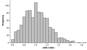 mean = 1.108, standard deviation = .2129
(h) 1.59 is a fair bit out in the tail of the distribution and appears to have a smallish p-value. If we count how many of these observations are 1.59 are larger (rounding down from 1.5911 so that 1.5911 is included), we find about 1% (10 out of 1000) of the simulated sample odds ratios are at least this extreme. This gives us some evidence, though not super strong of a relationship in the population.
(i) Example results:
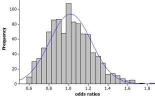
This distribution does not appear to be well-modeled by a normal curve.
(j) With a skewed right distribution, we can attempt a transformation. This will be appropriate if the transformed data follows a normal distribution. Then once we know the standard deviation of the normal model, we can construct a confidence interval.
(k) Example results
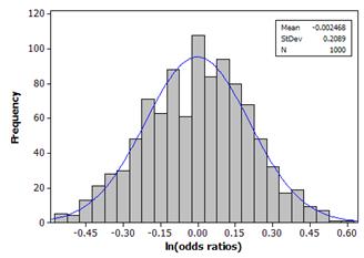 mean ≈ 0, SD =
.2089
mean ≈ 0, SD =
.2089
(l) Theoretical standard error:![]() = .2075
= .2075
This is very similar to the simulation results (SD = .2089)
(m) estimate + critical value × margin-of-error
ln(1.59) + 1.96(.2075) = .4637 + .4067 Þ (.057, .870)
exp(.057, .070) Þ (1.06, 2.39)
We are 95% confident that the odds of being in a car crash are 1.06 to 2.39 times larger for those without a full night’s sleep in the previous week compared to those with at least on full night’s sleep.
This interval does not capture one, so we have statistically significant evidence of an increase in odds for those without a full night’s sleep.
Optional:
If we calculate exp(ln(simulated odds ratio) + 1.96(.2075)) for each trial and then see whether or not one falls inside this interval (because in this simulation, we know that to be the value of the population odds ratio), then we hope to find roughly 95% of these interval include one.
Example results: .948
(n) Results from R
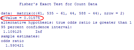
Note, this p-value is close to the 1% we simulated.
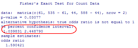
This is very close to the confidence interval we calculated.