INVESTIGATING STATISTICAL CONCEPTS, APPLICATIONS, AND METHODS, Second Edition

NOTES FOR INSTRUCTORS

January, 2015

Investigation 0: This can be used as an initial or “filler” exploration that focuses on the relative frequency interpretation of probability and using simulations to explore chance models. One key distinction you might want to emphasize for students is the estimated probability from simulation and the exact probability found analytically, which is not always so straight forward. There is also tremendous amount of flexibility on how deeply you want to go into probability rules, expected value, and variance. Many students don’t have a good understanding of what is meant by “simulation” so you may want to highlight that as you will return to the concept throughout the course. (You may even want to follow-up with additional simulation exercises, see Ch. 0 homework.) If you do the first part of this investigation in class, you probably want students bringing calculators as well. For the hands-on simulation, bring four index cards for each person or pair of students. The applet has been updated to javascript. You may want to watch/highlight use of the terms repetition vs. trial. A simpler case practice problem has been added. (If you use the applet for other than 4 babies, you will not see the animation.)

Some features of the textbook you may want to highlight include the glossary/index, links to applets, study conclusion boxes, and errata page. You should make sure students have access to the notes every day, either on their laptop or printed out, as they will want to add notes as they go along rather than having a separate notebook. You may also want to insist on a calculator every day. You will also want to make sure they have detailed instructions for the technology tools you want them to use in class (e.g., R or Minitab (version 16), ability to run javascript applets). In particular, you will want to make the ISCAM.RData workspace file available to R users. If you are using an R or Minitab-only version of the text, there will still be occasional mentions of the other package. You can use this as a reminder that there are other options, but generally ignore them. If using the pdf files, you should be able to copy and paste commands from the pdf into the technology.

CHAPTER 1

Section 1

This section will cover all the big ideas of a full statistical investigation: describing data, stating hypotheses, tests of significance, confidence intervals, and scope of conclusions. (Ideas of generalizability are raised but not focused on until later but you can bring in lots of statistical issues, like ethics, data snooping, types of error.) Once you finish this section, you may want to emphasize to students that the remaining material will cycle through these approaches with different methods. (In fact, you may want to reassure students that you are starting with some of the tougher ideas first to give them time to practice and reinforce the ideas.)

Investigation 1.1: Friend or Foe

Materials: You may want to bring some extra coins to class and/or tell students to in advance. The One Proportion applet is javascript and should run on all platforms. The applet initially assumes the coin tossing context for = 0.5 but then changes to spinners and “probability of success” more generally.

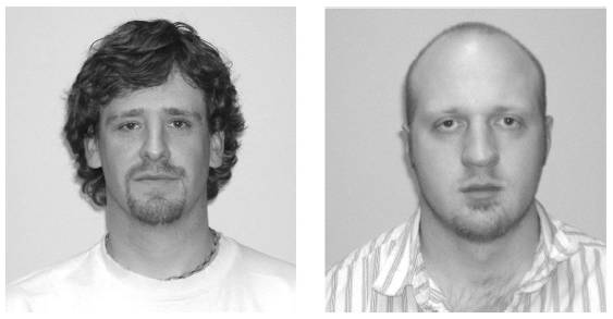
Timing: The entire activity takes about 80 minutes. A good place to split up the activity is after the applet (about 45 minutes) and before the mathematical model. You can then assign them to review the Terminology Detour before the next class. You may also want to collect data for the “matching faces” study (see link below), which so far we have found to work quite well in showing a tendency to agree on the name on the left, to have that data ready for Day 2.

We find this investigation a very good entry to the big ideas of the course. We encourage you to build up the design of the study (e.g., show the Videos) and highlight the overall reasoning process (proof by contradiction, evidence vs. proof, ruling out "random chance" as a plausible explanation, possible vs. plausible). Try not to let students get too bogged down in the study details (e.g., the researchers did rotate the colors, shapes, left/right side presentation, we are "modelling" each infant having the same probability, these infants may or may not be representative of all infants, etc.).

In question (a), you can emphasize that examining a graph of the observed data is our usual first step. In question (b), it works well to get students to think for themselves about possible explanations for the high number picking the helper toy. They can usually come up with: there is something to the theory or it was a huge coincidence. Now we have to decide between these explanations, but the random chance explanation is one that we can investigate. Depending on your class size, you may ask them to do fewer repetitions in question (g). You can also ask them to predict what they will see in the dotplot before it’s displayed. Try to give students time to work through the applet and begin to draw their conclusions. It will be important to emphasize to students why you are looking at the results for = .5, and how that will help address the research question. Students can usually get the idea that small p-values provide evidence against the “random chance alone” or “fluke” or “coincidence” explanation, and then warn them you will refine that interpretation as the course progresses. (But may want to highlight for them what the random component is in their probability calculation.) As you wrap up the activity you will want to focus on the reasoning behind the conclusion and precise phrasing of the conclusions. In particular, you may want to emphasize the distinction between interpreting the p-value and evaluating the p-value. The strategy outlined in the Summary gives a nice framework to the process (statistic, simulation, strength of evidence). You will especially want to repeatedly emphasize how the p-value is calculated assuming the null hypothesis is true. You may want to emphasize the “tail area” aspect of the p-value as a way to standardize the measurement of what’s unusual across different types of distributions (e.g., if we had a large sample size than any one outcome would have a low probability). You may want to poll a few students to report the p-value they estimated from the simulation to see that they vary slightly. This may motivate some students to want to calculate an “exact” answer that everyone should agree on, and this is certainly possible using a bit of probability theory.

After Practice Problem 1.1, there is an optional Probability Exploration that guides students to calculate the exact probability, followed by more “technical” details on this calculation. This also allows you to draw the distinction between the simulated p-value and the exact p-value. Having 2-3 methods for finding the p-value (exact vs. simulation vs. normal-model) will be a theme throughout the book. Another issue that may want to emphasize but may take getting used to is always defining the parameter as a process probability (rather than a population proportion). You may also choose to expand on the details and probability rules behind the binomial probability calculations.

The More Technical Details section is optional but offers one way to think about variability and tries to get students to think about variability “horizontally” rather than “vertically” and in terms of “consistency.” Students may have already heard about standard deviation or you may want to point them to references now. You can return to the idea of SD() when you cover those formulas with the normal approximation later.

Instructions for several uses of technology follow.

Loading data into R is one of the most difficult aspects so you may want to postpone that for later. Also make sure students see the question mark features with R and with the iscam R functions. The italics commands can be used to help identify the parameters being based into the functions.

For binomial calculations in R, you could of course use pbinom (e.g., 1-pbinom(13, 16, .5, TRUE) or pbinom(14, 16, .5, FALSE)), but we prefer the iscam function which includes the graph and uses non-strict inequalities for both tails.

In this version of the Minitab text we often include both command line and menu driven options. For the command line, you will need to remind students frequently about enabling commands or setting that up permanently.

Investigation 1.2: Matching Names to Faces

Materials: This works well to collect and analyze data on your students. A link to the pictures can be found here. We have tried randomizing the order of the faces/choices and have not found that to affect the results (but you may want to incorporate this into your data collection as well). A google docs type survey can work well here.

Technology: The text now assumes you will give them the summary data, but you might also want to get their feet wet reading the data in from a webpage or a URL (see technology detours at end of Investigation 1.1). With Minitab, you can copy and paste from the webpage into the data window (but watch that an extra missing value is not added to the end of the column). You will also want to make sure you introduce them to the “enable commands” menu. With R, you can use read.table or read.csv (for comma delimited). With R Studio, you can use Import Data > From Web URL. With R Markdown, you can use:

```{r}

Infats <- read.delim("http://www.rossmanchance.com/iscam2/data/InfantData.txt")

attach(Infants)

load(url("http://www.rossmanchance.com/iscam2/ISCAM.RData"))

```

to load in (tab delimited) data and the ISCAM workspace. You will also want to introduce students to “attaching” their data. To convert the * values to NaN, you can use as.numeric(as.character(x)). The materials make use of iscambinomtest which gives the output and graph together. You may want to compare this output to R's standard binom.test.

Timing: This investigation takes about 50 minutes of class time, not considering the data collection which can be completed inside or outside of class.

Students will gain practice in analyzing their own data, so make sure they have an easy way to access/import the data into the technology. Once students have the data file, they can work through the technology instructions on their own. You will also want to give students practice on the new terms in this investigation, as well as plenty of time to get used to the technology. Be sure to highlight the distinction between the unknown parameter and a conjectured value for the parameter, as well as the distinctions between parameter, statistic, and variable.

Practice Problem 1.2 is a nice review of these ideas and you could even highlight how the binomial is even more appropriate here where you have truly repeat observations from the same “process” rather than treating the individuals as “identical” when the observations come from different people, but that under the null hypotheses, the processes are the same. You can also draw the distinction between saying “she does better than guessing” and “she comprehends the problem elements.” You may also want to begin stressing the big idea of “making statements about the ‘world’ based on observing a sample of data” and that tests of significance “evaluate the strength of evidence against some claim about the world.”

Technology note: Students will be learning several different ways to do these calculations the first few days. You may want to move some of these calculations outside of class and have them submit their numerical answers between classes, but we mostly encourage you to let the technology handle the tedious calculations from this point on. For the ISCAM workspace functions, initially they are told to use the lower.tail feature, mimicking the more generic R functions, but then they will switch to “above/below” type inputs. (Some instructors prefer going straight to iscambinomtest.) Be sure to emphasize some of the subtle issues in R, like punctuation, continuing on to another line, short-cuts in the inputs, capitalization matters, etc.). You could use binom.test in R but again we prefer the automatic picture.

Investigation 1.3: Heart Transplant Mortality

Timing: This investigation is mostly review and may only take 15-30 minutes.

This investigation provides additional practice (but with a hypothesized probability other than 0.5) and highlights the different analysis approaches. Try to get students comfortable with the overall reasoning process but that there are alternative reasonable approaches to obtaining a p-value. You may want to focus on Ho as the "by chance" hypothesis (ho hum) and Ha as the research conjecture (a ha!). Also emphasize the distinction between St. George's (underlying) death rate and the observed proportion of deaths and the 0.15 value. You may want to emphasize the statistical thinking underlying this investigation – e.g., how we really shouldn’t reuse the initial data in testing the theory that the data pointed to. So ethnical issues, as well as the role of sample size, can be emphasized in discussing this activity. Students may struggle a bit with seeing these observations as a sample from some larger process with an underlying probability of “success.” Students will appreciate defining “death” as a “success” as is common in many epidemiological studies. The text also draws their attention to “failing to reject” null hypothesis versus “accepting the null hypothesis.”

The One Proportion Inference applet does have the option for showing the summary statistics (mean and standard deviation) of the simulated values, but we advise not to pay much attention to those details yet. You can also input only the probability of success, sample size, and value of interest, (press the Count button), and continue directly to the check the Exact Binomial box.

Investigation 1.4: Kissing the Right Way

Timing: 30 minutes, a good time for review or a quiz, but this investigation is more to set the stage for the next one.

This study provides an interesting context that can be used multiple times during the course. (There are tic-tac ads that make a similar claim if you want to display for students.) The main new idea here is a two-sided alternative. Students sometimes struggle with this idea, partly the motivation of looking in both tails, partly recognizing when a research question calls for a two-sided test. It is probably not worth spending much time on the "method of small p-values" other than to warn students that different packages may use slightly different algorithms. If you do want to talk more about it, you can point out that the answer varies depending on whether they start with 80 or 106 for the = 0.75 case. You may also want to go into a bit more detail on how the “expected value” is determined and what it means (perhaps tie back to Investigation 0). You may not like the “data snooping” emphasis here, which is not at all how these data would actually be analyzed, but our goal is (in the next investigation) to emphasize the logic of a confidence interval as an interval of plausible values for the parameter, especially if there is not a natural hypothesized value to test. Students will want lots of practice on recognizing when they should use a two-sided alternative (e.g., try to make this clear on the first few homeworks but then expect them to decide on their own later.) Also make sure they see examples/exercises where they fail to reject.

Investigation 1.5: Kissing the Right Way (cont.)

Timing: About 30-45 minutes

This investigation introduces students to the concept of interval estimation by asking them to construct a set of plausible values for the parameter based on inverting the (two-sided) test. Students often like to get into the “game” of seeing how close they can find the p-value to the cut-offs. The goal is also for students to see how that p-value changes as the hypothesized parameter moves away from the observed proportion (the R output provides a nice illustration of this but will need to be discussed with the students) and also the effect of the significance level on the interval. You may want to emphasize that the “inversion” necessary for these binomial intervals is actually pretty complicated and ends up being conservative because of the discreteness (when you plug in 0.05, it will return a value where the probability is at least 0.05). You may want to emphasize that they have now seen the two main inference methods – tests and intervals, and contrast the slightly different purposes of each.

Changing the parameter values individually is a bit clunky. You may want to wrap up with a nice visual such as this to drive the point home.

Is also a new version of the One Proportion applet that includes a slider for the probability of success. Test applet is here.

You can also highlight properties of confidence intervals (e.g., widen with confidence level, shorten with larger sample size), but these ideas will definitely come up in the next section as well.

I recently changed the R functions (binomtest, onepropz, twopropz, onesamplet) so that if you enter multiple confidence levels, e.g., iscambinomtest(11, 20, conf.level = c(.90, .95)) it will display the intervals together in the output window.

Investigation 1.6: Improved Batting Averages

Timing: The full version of this is probably 90 minutes, but can be made much shorter, especially if don’t go through the calculation details. Students often struggle with this topic so you will want to think carefully about how much you want to emphasize it.

Materials: The Power applet has been updated to javascript. There is also a function in the ISCAM workspace that will do the entire power calculation (iscambinompower), but you may prefer not to mention that with students.

This investigation focuses on the idea of power, first through simulation, and then on the calculations of power using the binomial model. Students often struggle with the “two-step” approach to calculating power. One possible stopping point is after question (x) and there is a practice problem there (1.6A) focusing on the definitions. If you want students to do the calculations themselves, make sure you are focusing on the "we are doing this because" parts of the calculation steps. You can then focus on one the main purpose of power calculations – sample size determination.

We encourage you to give students a chance to struggle with the calculations a bit before modelling the full approach. You may want to give them empty screen captures of the technology to make sure they know what pieces to fill in to get the desired calculations. For more practice, make sure they can do greater than and less than alternative hypotheses. You may also want to give them even more pictures than what is in the text, especially in illustrating the factors that affect the calculations (e.g., http://statweb.calpoly.edu/bchance/stat301/power.html - click in lower right corner).

Section 2

This section reviews the previous material but through the “traditional” computational model – the normal distribution. This audience appears capable of working with the normal model without a lot of background detail, but some will be helpful when you get to critical values and if you cover the continuity correction ideas. (You may want to detour with some traditional normal probability model calculations for practice.) Try to emphasize the parallels with the previous methods (simulation, exact binomial), the correspondence between the binomial and normal results, and some tongue-in-cheek that these normal-based methods aren’t really necessary anymore with modern computing. Although students may appreciate the simplification in some of the calculations, in particular how to improve the calculation of confidence intervals.

Investigation 1.7: Reese’s Pieces

Timing: This activity will probably go across two class periods, about 90 minutes. You can assign the definition boxes for outside of class.

Technology: The Reese’s Pieces applet is now java-script. The "Show previous" box in the applet will allow you to compare the current distribution to results from the previous settings.

The beginning of this activity is largely review, but students will appreciate the candies. The fun size bags of Reese's work well, or you can bring dixie cups and fill them up individually. We would continue to stress the distinction between the sample data for each student (e.g., the bar graphs) and the accumulated class data (the sampling distribution). You may want to adopt a catchy term for the latter distribution such as "what if" (what if the null had been true) or "null" distribution. (We use "could have been" to refer to an individual simulated sample in these early investigations but not throughout the course.) Once you get to the applet, the focus is on how the parameters (and n) change the picture and you may want to look at some extreme cases as well to see different shapes and discreteness. The last half of the investigation works well as more of a lecture. If you have time, you may want to do more to derive the standard deviation formula using rules for variances of random variables. The Reese's applet now has a feature that displays the normal distribution’s probability value as well. That visual will help emphasize the continued focus on how to interpret a p-value in terms of the percentage of samples with a result at least that extreme (under the hypothesized probability).

Many students, but not all, will have some familiarity with standard deviation and for now we only give them the loose interpretation in the first Definition box. A simple demo of the properties of the mean and SD can be found here. An overview of the theoretical proof of these results can be found here. You may also want to assign homework that has them look at how the SD formula changes (e.g., play with derivatives) with changes in n and (especially maximizing at = 0.5). This is a great time to tie the empirical rule (focus on 2 standard deviations) to the common cut-off value for p-values of 0.05. (You will want to highlight this through the next few investigations leading up to the idea of a confidence interval.) You may also want to detour to general practice with normal probability calculations (for quantitative variables).

Investigation 1.8: Is ESP Real?

Timing: 30 minutes if you go through it mostly together, focusing on “putting the pieces together”

Students should be able to understand this context fairly quickly or this is a good one to assign the background for them to read in advance. (You may choose to show/assign some videos as well.) This investigation provides practice in using the Normal Distribution for calculating probabilities of sample proportions. Make sure they understand how to use the technology to look at two different values and finding the probability “outside.” Continue to focus on interpreting the calculations. You may have time to do some of the practice in class and/or spend more time on z-score. You may need to spend a few minutes justifying the use of the normal model as an alternative (approximate) model and the z-score provides one advantage and confidence intervals will provide a strong second one (and even power calculations). Math majors will also appreciate seeing how the factors affecting the p-value show up in the formulas. Make sure they see the study conclusions and definition boxes at the end of the investigation (one option is to assign and discuss Practice Problem 1.8 before showing them the z-score definition, they pick up this concept fairly quickly).

Technology hint: You may want to make sure they can use their technology to find probabilities “between” and/or “outside” two values.

Investigation 1.9: Halloween Treat Choices

Timing: 45-60 minutes, especially if they are familiar with the study context in advance (you might even want to assign parts (a)-(c) to be completed before class)

Students will practice applying the CLT and we recommend giving them several minutes on their own in part (f). Make sure they see the link to Ho and Ha (and ₀). You can also discuss why the z value is positive/negative and the short cuts they can take with a symmetric distribution. The definition of a test statistic is really the only new idea here. In (l)-(n) you will have to caution them against "proving" the null and also that they are talking about the process in general vs. individual children. You may want to try to get them in the habit of telling you the inputs to the technology they are using. It is pretty amazing how much the continuity correction helps and you will want to refer to earlier pictures in explaining it. Make sure students understand when you add or subtract the correction term, but otherwise you may not want to spend much time on the correction. (The Theory-Based Inference applet has a check box for this correct, adjusting both the z-value and the p-value.) It does force them to think deeply about many of the earlier ideas in the course (e.g., continuous vs. discrete and shape, center, and spread, strict inequalities). Question (r) is trickier than it sounds – the best approach is to return to the CLT normal distribution and find the probabilities for > 148.5/284 =.523 and < 135.5/284 = .477. You can now find a normal approximation using the One Proportion applet and you may want to show them the effects of the continuity correction visually.

This investigation also introduces the concept of checking the validity of a procedure. You will want to emphasize some “code language” for students to know that is what you are referring to as you proceed through the course (e.g., validity checks, technical conditions).

The practice problems here revisit the idea of power and you may want to introduce calculations here if you haven’t before as they can be a bit simpler. (This also provides a great extension for an exam if you don’t cover it in class.) Students may interpreted what is meant by each region differently (e.g., needing to combine I and III together). Make sure they don’t miss the study conclusions box and the overall Summary of One Sample z-Test box.

Investigation 1.10: Kissing the Right Way (cont.)

Timing: 45-60 minutes

This investigation introduces the one proportion z-interval and you have some options as to how much detail you want to include (e.g., finding percentiles). Students may need more guidance in coming up with critical values. You will also want to discuss how this interval procedure relates to what they did before and to the general ± 2 SD form. (This will hopefully provide some motivation for the normal model.) They will need some guidance on question (d) and how we can think of 2 standard deviations as a maximum plausible distance. Students seem to do well with this “two standard deviation rule.” Try to get students to think in terms of the formula in (h) versus a specific calculated interval. When you get to the Simulating Confidence Intervals applet, students can work through most of this on their own, just make sure they notice the “Running Total” output. It works best to generate 200 intervals at a time and then accumulate to 1000. Also have them think about what it means for the interval to be narrower - what that implies in response to the research question. Not clear how much time you want to spend on sample size determination but student intuition here is rather poor. Also, if not covered before, they will need to realize that the SD formula is maximized when the proportion equals 0.5. Question (n) is a bit open in what they choose to use for (e.g., 0.645 from the previous study or 0.5 to be safe, or both and contrast, or their own guess). It can be nice to show how the binomial intervals are a bit longer and not symmetric. You will also need to decide how much emphasis you want to put on the frequentist interpretation of confidence level and the idea of “reliability” of a method. Students will need lots of practice and feedback, even in recognizing when the question asks about interpretation of the interval vs. interpretation of the confidence level.

You may also want to make them think carefully about the difference between standard deviation and standard error at this point. The practice problem in this investigation can be split into pieces (e.g., you may want to save c and d for after Investigation 1.11 which does not have a practice problem).

Investigation 1.11: Hospital Mortality Rates (cont.)

Timing: This can be done in combination with other activities and may take 15-30 minutes (it can tie in nicely with a review of the Wald interval and Wald vs. binomial intervals and how to decide between procedures). You may have time at the end of a class period to collect their sample data for the first part of the next investigation (choosing 10 “representative” words).

Many statisticians now feel only the “plus four” method should be taught. We prefer to start with the traditional method for its intuition (estimate + margin of error) but do feel it’s important for students to see and understand the goals of this modern approach. You can also highlight to students how they are using a method that has gained in popularity in the last 20 years vs. some of their other courses which only use methods that are centuries old. Make sure students don't get bogged down by the numerous methods but gain some insight into how we might decide one method is doing “better” than another or not.

Do make sure you use 95% confidence in the Simulating Confidence Intervals applet with the Adjusted Wald – it may not use the fancier adjustment with other confidence interval levels. (It’s also illuminating to Sort the intervals and see the intervals with zero length with = 0 for the Wald method.) Then let them practice on calculating the Adjusted Wald in (g), making sure students remember to increase n in the denominator as well as using the adjusted estimate. You may also want to assign a simple calculation practice for a practice problem to this investigation or focus on benefits/disadvantages of the procedures.

Section 3

There is a minor transition here to focusing on samples from a population rather than samples from a process. It may be worth defining a process for them to help them see the distinction. The goal is to help them quickly see that they will be able to apply the same analysis tools but now we will really consider whether or not we can generalize our conclusions to a larger population.

Investigation 1.12: Sampling Words

Timing: About 30 minutes and can probably be combined with 1.13 in one class period.

Students may not like the vagueness of the directions and you can tell them that you want the words in the sample to give you information about the population. In fact, we claim that even if you tell them you are trying to estimate the lengths of the words, you will still get bias. This will also be students' first consideration of quantitative variables in a while. We recommend getting students up and out of their seats to share their results for at least one of the distributions. If using the ISCAM workspace in a lab, do be cautious that everyone may have the same seed! (You can remove the seed first.) Although the Central Limit Theorem for a sample mean is not officially discussed for a while, you may want to make many of those points here and note them for later use, or even preview the result at this time. Earlier we said we were most interested in the standard deviation of the simulated distribution. Here you can contrast with focusing on the mean for judging bias.

A nice extension to this activity if you have time is to consider stratified sampling and have them see the sampling distribution with less sampling variability (see Chapter 1 Appendix for brief introduction to this idea).

For practice problem 1.12A, consider whether or not you want students to write out the explanations for their answers. You might also again emphasize the distinction between the distribution of the sample and the distribution of the sample statistics.

Investigation 1.13: Literary Digest

Timing: 10 minutes as a class discussion or assigned as homework.

This famous example is an opportunity to practice with the new terms. Can also embellish with lots of historical fun facts as well- for example:

GEORGE GALLUP, JR.: It had been around in academic settings and so forth, and Roper had started the Fortune Poll a few months earlier. And so, there were sporadic efforts to do it, but my dad brought it to the national scene through a syndicated newspaper service, actually. Well, the reaction to that first report was dismay among New Dealers, of course, and the attacks started immediately. How can you interview merely - I think in those days it was two or three thousand people - and project this to the entire country.

That began to change, actually, the next year, when Gallup, Roper and Crossley, Archibald Crossley was a pollster, and Elmo Roper was another pollster, these were the three scientific pollsters, if you will, operating in 1936, and their success in the election, and the failure of the Literary Digest really changed some minds. And people started to think, well, maybe polls are accurate after all.

From Wikipedia:

In 1936, his new organization achieved national recognition by correctly predicting, from the replies of only 5,000 respondents, the result of that year’s presidential election, in contradiction to the widely respected Literary Digest magazine whose much more extensive poll based on over two million returned questionnaires got the result wrong. Not only did he get the election right, he correctly predicted the results of the Literary Digest poll as well using a random sample smaller than theirs but chosen to match it. …

You can also touch on nonsampling errors with Gallup or the more recent New Hampshire primary between Clinton and Obama.

Twelve years later, his organization had its moment of greatest ignominy, when it predicted that Thomas Dewey would defeat Harry S. Truman in the 1948 election, by five to 15 percentage points. Gallup believed the error was mostly due to ending his polling three weeks before Election Day.

Here is an excerpt from Gallup.com on how they conduct a national poll that illustrates all of these points!

Results are based on telephone interviews with 1,014 national adults, aged 18 and older, conducted March 25, 2009. ….

Polls conducted entirely in one day, such as this one, are subject to additional error or bias not found in polls conducted over several days.

Interviews are conducted with respondents on land-line telephones (for respondents with a land-line telephone) and cellular phones (for respondents who are cell-phone only).

In addition to sampling error, question wording and practical difficulties in conducting surveys can introduce error or bias into the findings of public opinion polls.

You may want to end with follow-up discussion on how non-random samples may or may not still be representative depending on the variable(s) being measured.

Investigation 1.14: Sampling Words (cont.)

Timing: 30 minutes (this can be done instead of or in addition to Investigation 1.15 or skipped for Investigation 1.15)

This works well as a class discussion. You will want to again emphasize to students that this is one of the rare cases where we have the entire population and our goal is to investigate properties of the procedures so that we can better understand what they are telling us in actual research studies. You will also want to empathize with students how counter intuitive the population size result is. You can also remind them of the parallels to sampling from a process. You will definitely want to at least mention Investigation 1.15 and the idea of a finite population correction factor.

The main thing to help them with is that the first distribution turns green when the next distribution is overlaid on it. They won’t see much difference in these distributions and you can compare the mean and SD values as well. Students seem to have a hard time “accepting” this result so you will want to make a big deal out of it.

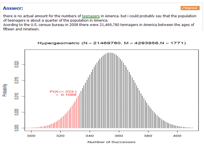
Investigation 1.15: Freshmen Voting Pattern

This investigation introduces the hypergeometric distribution as a model for sampling from a finite population. This investigation is definitely skippable and you won’t want to spend too much time on the hypergeometric at this time, but you can show them how the binomial distribution is a reasonable approximation when the population size is large (tying back to what they saw in Investigation 1.14).

A second key idea in this investigation is nonsampling errors. These are also referenced in one of the chapter examples.

Investigation 1.16: Teen Hearing Loss

Timing: 15 minutes

This investigation again provides practice with the new terms and gets students back to the inferential world. You may want to compare the binomial calculations with the “exact” hypergeometric calculations, and even show the insensitivity of this calculation to the population size if the population proportion is held constant.

Investigation 1.17: Cat Households

Timing: About 15 minutes. Students should be able to complete 1.17 and 1.18 largely on their own in one class period. They also work well as homework exercises.

This is a quick investigation to draw students' attention to the difference between statistical and practice significance.

Investigation 1.18: Female Senators

Timing: About 15 minutes.

Another quick investigation with an important reminder. You will get a lot of students to say yes to (d).

End of Chapter

Definitely draw students’ attention to the examples. The goal is for them to attempt the problems first, and then have detailed explanations available. Note that non-sampling errors are formally introduced in Example 1.3. The chapter concludes with a Chapter Summary, a bullet list of key ideas, and a technology summary.