Chapter 6

This chapter again extends the lessons students have learned in earlier chapters to additional methods involving more than one variable. The material focuses on the new methods (e.g., chi-square tests, ANOVA, and regression) and follows the same progression as earlier topics: starting with including appropriate numerical and graphical summaries, proceeding to use simulations to construct empirical sampling/randomization distributions, and then considering probability models for drawing inferences. The material is fairly flexible if you want to pick and choose topics. Fuller treatments of these methods would require a second course.

Section 6.1: Two Categorical Variables

Timing/materials: Minitab and a macro (SpockSim.mtb) are used in Investigation 6.1.1. Minitab is used to carry out a chi-square analysis in Investigations 6.1.2 and 6.1.3. These three investigations may take about 90-100 minutes, with Investigation 6.1.1 taking about 50-60 minutes. Exploration 6.1 revolves around a Minitab macro (twoway.mtb which uses worksheet refraction.mtw).

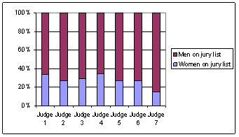
The focus of this section is on studies involving two categorical variables and in particular highlights different versions of the chi-square test for tables larger than 2 × 2. In Investigation 6.1.1 you may want to spend a bit of time on the background process of the jury selection before students analyze the data. We also encourage you again to stop and discuss the numerical and graphical summaries that apply to these sample data (question (a)) before proceeding to inferential statements, as well as reconsidering the constant theme – could differences this large have plausibly occurred by chance alone? After question (h), you will also want to explain the logic behind the chi-square statistic – every cell gives a positive contribution to the sum but it is also scaled in a way by the size of the cell’s expected cell count. If students follow the formula, question (j) should be straight forward to them. After thinking about the behavior based on the formula, we then use simulation as a way of judging what values of the statistic should be considered large enough to be unusual and also to see what probability distribution might approximate the sampling distribution of the test statistic. Because we are simulating the drawing of independent random samples from several populations, we use the binomial distribution, as opposed to treating both margins as fixed like we did in Chapter 1. We have given students the macro to run (SpockSim.mtb) in question (k), but you may want to spend time making sure they understand the workings of the Minitab commands involved and the resulting output. The simulation results are also used to help students see that the normal distribution does not provide a reasonable model of the empirical sampling distribution of this test statistic. We do not derive the chi-square distribution but do use probability plots to show that the Gamma distribution, of which the chi-square distribution is a special case, is appropriate (questions (n) and (o)). Again, we want them to realize that the probability model applies no matter the true value of the common population proportion p. We also encourage them to follow-up a significant chi-square statistic by seeing which cells of the table contribute the most to the chi-square sum as a way of further defining the source(s) of discrepancy (questions (q) and (r)). There is a summary of this procedure on p. 490 along with Minitab instructions. The section of Type I Errors on p. 491 is used to further motivate the use of this “multi-sided” procedure for checking the equality of all population proportions simultaneously.

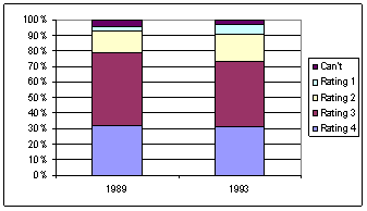
Investigation 6.1.2 provides an application of the chi-square procedure using Minitab but in the case of a cross-classified study first examined in Chapter 1. You might want to start by asking them what the segmented bar graph would have looked like if there was no association between the two variables. The details of the chi-square procedure are summarized, with Minitab instructions, on p. 494-5 and you may wish to give students additional practice, in addition to the practice problems, especially in distinguishing these different situations, (e.g., reminding them of the different data collection scenarios, the segmented bar graphs, the form of the hypotheses – comparing more than 2 population proportions, comparing population distributions on a categorical variable, association between categorical variables).

Investigation 6.1.3 focuses on the correspondence between the chi-square procedure for a 2 × 2 table and the two-sample z-test with a two-sided alternative.

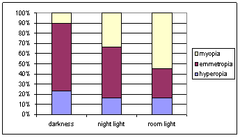
Exploration 6.1 may be considered optional but is meant to illustrate that the chi-square distribution is appropriate for modeling the randomization distribution (corresponding to Investigation 6.1.2) as well as the sampling distribution (as in Investigation 6.1.1). Students are given a macro to run but are asked to explain the individual commands.

Section 6.2: Comparing Several Population Means

Timing/materials: Minitab is used for descriptive statistics (HandicapEmployment.mtw) and a Minitab macro (RandomHandicap.mtb) is used in Investigation 6.2.1. Minitab is used again at the end of the investigation to carry out the ANOVA. Minitab can be used briefly in Investigation 6.2.2 to calculate a p-value from the F distribution. The ANOVA simulation applet is also used heavily. This section should take about 65 minutes.

The focus on this section is on comparing 2 or more population means (or treatment means). You may want to cast this as the association between one categorical and one quantitative variable to parallel the previous section (though some suggest only applying this description with cross-classified studies). Again, we do not spend a large amount of time developing the details, seeing these analyses as straight forward implementations of previous tools with slight changes in the details of the calculation of a test statistic. We hope that students are well-prepared at this point to understand the reasoning behind the big idea of comparing within-group to between-group variation, but you might want to spend some extra time on this principle. You will also want to focus on emphasizing all the steps of a statistical analysis (examination of study design, numerical and graphical summaries, and statistical inference including defining the parameters of interest, stating the hypotheses, commenting on the technical conditions, calculation of test statistic and p-value, making a decision about the null hypothesis, and then finally stating an overall conclusion that touches on each of the issues).

Investigation 6.2.1 steps students through the calculations and comparison of within group and between group variability and uses a macro to examine the empirical sampling distribution of the test statistic. Question (o) is a key one for assessing whether students understand the basic principle. More details are supplied in the terminology detour on p. 506 and general Minitab instructions for carrying out an ANOVA analysis are given on p. 507.

In Investigation 6.2.2, students initially practice calculating the F-statistic by hand. Then a java applet is used to explore the effects of sample size, size of the difference in population means, and the common population variance on the ANOVA table and p-value. We have tried to use values that allow sufficient sensitivity in the applet to see some useful relationships. It is interesting for students to see the variability in the F-statistic and p-value from sample to sample both when the null hypothesis is true and when it is false. An interesting extension would be to collect the p-values from different random samples and examine a graph of their distribution, having students conjecture on its shape first.

Practice Problem 6.2.1 is worth emphasizing; its goal is to help students understand why we need a new procedure (ANOVA) here in the first place, as opposed to simply conducting a bunch of two-sample t-tests on all pairs of groups. Practice Problem 6.2.2 demonstrates the correspondence of ANOVA to a two-sided two-sample t-test, when only two groups are being compared, and is worth highlighting. An interesting in-class experiment to consider in the section on ANOVA is the melting time of different types of chips (e.g., milk chocolate vs. peanut butter vs. semi-sweet, similar to the study described in Exercise 46 in Chapter 3), especially considering each person as a blocking factor (and are willing to discuss “two-way” ANVOA). You might also consider at least demonstrating multiple comparison procedures to your students.

Exercise 59 is a particularly interesting follow-up question, re-analyzing the Spock trial data using ANOVA instead of Chi-square, and considering how the two analyses differ in the information provided.

Section 6.3: Relationships Between Quantitative Variables

Timing/materials: Minitab is used for basic univariate and bivariate graphs and numerical summaries in Investigation 6.3.1 (housing.mtw). Minitab is used to calculate correlation coefficients in Investigation 6.3.2 (golfers.mtw). These two investigations may take about 45 minutes. Exploration 6.3.1 revolves around the Guess the Correlation applet and will take 10-15 minutes. Investigation 6.3.3 uses the Least Squares Regression applet and at the end shows them how to determine a regression equation in Minitab (HeightFoot.mtw) and can take upwards of 60 minutes. Investigation 6.3.4 also involves Minitab (movies03.mtw) and may take 30 minutes. Exploration 6.3.2 revolves around the Least Squares Regression applet and Exploration 6.3.3 uses Minitab (BritishOpen00.mtw).

This section presents tools for numerical and graphical summaries in the setting of two quantitative variables. Here we are generally less concerned about the type of study used. The next section will focus on inference for regression.

Investigation 6.3.1 focuses on using Minitab to create scatterplots and then introducing appropriate terminology for describing them. Investigation 6.3.2 uses data from the same source (PGA golfers) to explore varying strengths of linear relationships and then introduces the correlation coefficient as a measure of that strength. One thing to be sure that students understand is that low scores are better than high scores in golf; similarly a smaller value for average number of putts per hole is better than a larger value, but some other variables (like driving distance) have the property that higher numbers are generally considered better. Discussion in this investigation includes how the points line up in different quadrants as a way of visualizing the strength of the linear relationship. Question (i) is a particularly good one to give students a few minutes to work through on their own in collaborative groups. Students should also be able to describe properties of the formula for r (when positive, negative, maximum and minimum values, etc.); in fact, our hope in (k)-(n) is that students can quickly tell you these properties rather than you telling them. Students apply this reasoning to order several scatterplots in terms of strength and then use Minitab to verify their ordering. If you want students to have more practice in estimating the size of the correlation coefficient from a scatterplot, Exploration 6.3.1 generates random scatterplots, allows students to specify a guess for r and then shows them the actual value. The applet keeps track of their guesses over time (to see if they improve) as well as the guesses vs. actual and errors vs. actual to see which values of r were easier to identify (e.g., closer to -1 and 1). Questions (g)-(i) also get students to think a bit about the meaning of r. Students often believe they are poor guessers and that the correlation between their guesses and the actual values of r will be small. They are often surprised at how high this correlation is, but should realize that this will happen as long as they can distinguish positive and negative correlations and that they may find a high correlation if they guess wrongly in a consistent manner. Practice Problem 6.3.1 is a very quick test of students’ understanding; question (b) in particular confuses many students. A Practice Problem like 6.3.2 is important for reminding them that r measures the amount of the linear association.

Investigation 6.3.3 steps students through a development of least squares regression. Starting after (g), they use a java applet with a moveable line feature to explore “fitting the best line” and realize that finding THE best line is nontrivial and even ambiguous, as there are many reasonable ways to measure “fit.” We emphasize the idea of a residual, the vertical distance between a point and the line, as the foundation for measuring fit, since prediction is a chief use of regression. In question (k) we briefly ask students to consider the sum of absolute residuals as a criterion, and then we justify using SSE as a measure of the prediction errors. Parallels can be drawn to Exploration 2.1 (p. 133). In questions (k)-(m) many students enjoy the competitive aspect of trying to come up with better and better lines according to the two criteria. Students can then use calculus to derive the least squares estimators directly in (p) and (q). Questions (s) and (t) develop the interpretation of the slope coefficient and question (u) focuses on the intercept. Question (v) warns them about making extrapolations from the data. The applet is then used in questions (w) and (x) to motive the interpretation of r². Spacing left in the book for written responses to these questions is probably smaller than it should be. Once the by-hand derivation of the least squares estimates are discussed, instructions are given for obtaining them in Minitab. Investigation 6.3.4 provides practice in determining and interpreting regression coefficients with the additional aspect, which students often find interesting, of comparing the relationship across different types of movies.

Exploration 6.3.2 uses an applet to help students visualize the influence of data values, particularly those with large x-values, on the regression line. Exploration 6.3.3 introduces students to the “regression effect.” There is a nice history to this feature of regression and it also provides additional cautions to students about drawing too strong of conclusions from their observations (e.g., “regression to the mean”). We often supplement this discussion with excerpts from the January 21, 2001 Sports Illustrated article on the cover jinx.

“It was a hoot to work on the piece. On the one hand, we listened as sober statisticians went over the basics of ‘regression to the mean,’ which would explain why a hitter who gets hot enough to make the cover goes into a slump shortly thereafter.”

Section 6.4: Inference for Regression

Timing/materials: Minitab is used in Investigation 6.4.1 (hypoHt.mtw) and Investigation 6.4.2 (housing.mtw). Together, these investigations can take less than 30 minutes. Investigation 6.4.3 revolves around the Simulating Regression Lines applet and takes 35-45 minutes. Investigation 6.4.4 really just requires a calculator (Minitab output is supplied) and takes about 20 minutes.

This section finishes the discussion of regression by developing tools to make inferential statements about a population regression slope. Investigation 6.4.1 begins by having students consider the “ideal” setting for such inferences – normal populations with equal variance that differ only in their means that follow a linear pattern with the explanatory variable. We especially advocate the LINE mnemonic. Residual plots are introduced as a method for checking the appropriateness of this basic regression model. Investigation 6.4.2 then applies this model to some student collected data. The linearity condition does not appear met with these data and we have them perform a log-log transformation. If you think this transition will be too challenging for your students, you may want to provide more linear examples first. Details for why the log-log transformation is appropriate and for interpreting the resulting regression coefficients in terms of the original variables are left for a second course. In this section we are more concerned that students can check the conditions and realize that additional steps can be taken when they are not met and we try not to get too bogged down at this time in interpreting the transformation.

Investigation 6.4.3 follows the strategy that we have used throughout the course: taking repeated random samples from a finite population in order to examine the sampling distribution of the relevant sample statistic. We ask students to use a java applet to select random samples from a hypothetical population matching the house price setting that follows the basic regression model, but where the population has been chosen so that the correlation (and therefore the slope) between log(price) and log(size) is zero. The goal of the applet is for students to visualize sampling variability with regression slopes (and lines) as well as the empirical sampling distribution of the sample slopes. This process should feel very familiar to students at this point, although you should be aware that it feels different to some students because they are watching sample regression lines change rather than seeing simpler statistics such as sample proportions or sample means change. Students also explore the effects of sample size, variability in the explanatory variable and variability about the regression line on this sampling distribution. This motivates the formula for the standard error of the sample slopes given on p. 550. It is interesting to help students realize that when choosing the x values, as in an experiment, more variability in the explanatory variable is preferred, a sometimes counter-intuitive result for them. Students should also note the symmetry of the sampling distribution of sample slope coefficients and believe that a t-distribution will provide a reasonable model for the standardized slopes using an estimate for the standard deviation about the regression line. Students calculate the corresponding t-statistic for the house price data by hand.

Investigation 6.4.4 then further focuses on the corresponding Minitab output. Questions (f)-(l) also deal with confidence intervals for slope and confidence intervals and prediction intervals (and the distinction between them, for which you can draw the connection to univariate prediction intervals from Chapter 4) for individual values. Minitab provides for nice visuals for these latter intervals. The bow-tie shape they saw in the applet is also a nice visual here for justifying the “curvature” seen especially in prediction intervals.

Examples

This chapter includes four worked-out examples. Each of the first three deals with one of the three main methods covered in this chapter: chi-square tests, ANOVA, and regression. The fourth example analyzes data from a diet comparison study, where we ask several questions and expect students to first identify which method applies to a given question. Again we encourage students to answer the questions and analyze the data themselves before reading the model solutions.

Summary

At the end of this chapter, students will most need guidance on when to use each of the different methods. The table on p. 571 may be useful but students will also need practice identifying the proper procedure merely from a description of the study design and variables. We also like to remind students to be very conscious of the technical conditions underlying each procedure and that they must be checked and commented on in any analysis.

Exercises

Section 6.1 issues are addressed in Exercises #1-16 and #61.  Section 6.2 issues are addressed in Exercises #17-30 and #59 and #62.  Section 6.3 and 6.4 issues are addressed in Exercises #31-60 and #63.  Exercises #60-62 ask students to perform all three types of analyses (chi-square, ANOVA, regression) on the same set of data, and Exercise #59 asks for an ANOVA analysis of data previously analyzed with a chi-square procedure. NOTE: The data file for “ComparingDietsFull.mtw” on the CD does not contain all of the necessary variables to complete Exercise 29. A newer version of the data file can be download from the ISCAM Data Files page.