Chapter 3

In this chapter, we transition from comparing two groups to focusing on how to sample the observational units from a population. While issues of generalizing from the sample to the population were touched in Chapter 1, in this chapter students formally learn about random sampling. We focus (but not exclusively) on categorical variables and introduce the binomial probability distribution in this chapter, along with more ideas and notation of significance testing. There is a new spate of terminology that you will want to ensure students have sufficient practice applying. In particular, we try hard to help students clearly distinguish between the processes of random sampling and randomization, as well as the goals and implications of each.

Section 3.1: Sampling from Populations I

Timing/Materials: Investigation 3.1.1 should take about one hour. We encourage you to have students use Minitab to select the random samples but they can also use the calculator or a random number table (if supplied). Investigation 3.1.2 can be discussed together quickly at the end of a class period, about 15 minutes. An applet is used in Investigation 3.1.3 and there are some Minitab questions in Investigation 3.1.4. These two investigations together probably take 60-75 minutes. You will probably want students to be able to use Minitab in Investigation 3.1.5 which can take 30-40 minutes. Exploration 3.1 is a Minitab exercise focusing on properties of different sampling methods (e.g., stratified sampling) which could be moved outside of class (about 30 minutes) or skipped. Investigation 3.1.2 and Exploration 3.1 can be regarded as optional if you are short on time.

The goal of Investigation 3.1.1 is to convince students of the need for (statistical) random sampling rather than convenience sampling or human judgment. Some students want to quibble that part (a) only asks for “representative words” which they interpret as indicating representing language from the time or words conveying the meaning of the speech. This allows you to discuss that we mean “representative” as having the same characteristics of the population, regardless of which characteristics you will decide to focus on. Here we focus on length of words, expecting most students to oversample the longer words. Through constructing the dotplot of their initial sample means (again, we usually have students come to the front of the class to add their own observation), we also hope to provide students with a visual image of bias, with almost all of the student averages falling above the population average. We hope having students construct graphs of their sample data (in (d)) prior to the empirical sampling distribution (in (k)) will help them distinguish between these distributions. You will want to point out this distinction frequently (as well as insisting on proper horizontal labels of the variable for each graph – word length in (d) and average word length in (k)). We think it’s especially important and helpful to emphasize that the observational units in (d) are the words themselves, but the observational units in (k) are the students’ samples of words- this is a difficult but important conceptual leap for students to make. The sampling distribution of the sample proportions of long words in (k), due to the small sample size and granularity may not produce as a dramatic an illustration of bias, but will still help get students thinking about sampling distributions and sampling variability. This investigation also helps students practice with the new terminology and notation related to parameters and statistics. We often encourage students to remember that the population parameters are denoted by Greek letters, as in real applications they are unknown to the researchers (“It’s Greek to me!”). The goals of questions (r)-(w) are to show students that random sampling does not eliminate sampling variability but does eliminate bias by moving the center of the sampling distribution to the parameter of interest. By question (w) students should believe that a method using a small random sample is better than using larger nonrandom samples. Practice 3.1.1 uses a well-known historical context to drive this point home (You can also discuss Gallup’s ability to predict both the Digest results and the actual election results much more accurately with a smaller sample).

Investigation 3.1.2 is meant as a quick introduction to alternative sampling methods – systematic, multistage, and stratified. This investigation is optional, but you may even choose to talk students through these ideas but it’s useful for them to consider methods that are still statistically random but that may be more convenient to use in practice.

In the remainder of the text, we do not consider how to make inferences from any sampling techniques other than simple random sampling.

Investigation 3.1.3 introduces students to the second key advantage of using random sampling: not only does it eliminate bias, but it also allows us to quantify how far we expect sample results to fall from population values. This investigation continues the exploration of samples of words from the Gettysburg address using a java applet to take a much larger number of samples and to more easily change the sample size in exploring the sampling distribution of the sample mean. Students should also get the visual for a third distribution (beyond the sample and the empirical sampling distribution), the population. The questions step students through the sampling process in the applet very slowly to ensure that they understand what the output of the applet represents (e.g., what does each green square involve). The focus here is on the fundamental phenomenon of sampling variability, and on the effect of sample size on sampling variability; we are not leading students to the Central Limit Theorem quite yet. A common student difficulty is distinguishing between the sample size and the number of samples so you will want to discuss that frequently. 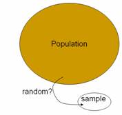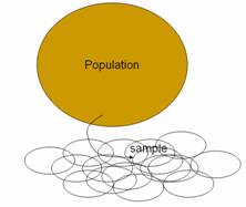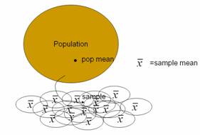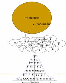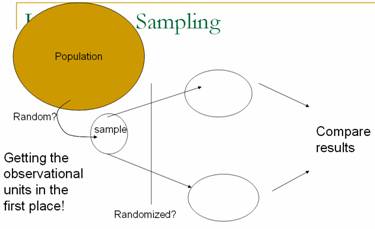Questions (m)-(p) attempt to help students to continue to think in terms of statistical significance by asking if certain sample results would be surprising; this reinforces the idea of an empirical p-value that arose in both Chapters 1 and 2. You may consider a simple PowerPoint illustration to help them focus on the overall process behind a sampling distribution (copy here), e.g.:

This exploration is continued in Investigation 3.1.4 but for sample proportions. Again the focus is on exploring sampling variability and sample size effects through the applet simulation. Beginning in (e) students are to see that the hypergeometric probability distribution describes the exact sampling distribution in this case. Students again use Minitab to construct the theoretical sampling distribution and expected value which they can compare to the applet simulation results. Students continue this comparison by calculating the exact probability of certain values compared to the proportion of samples simulated. Questions (o) and (p) ask students to again consider questions of what inferences can be drawn from such probability calculations. The subsequent practice problems address another common student misconception, that the size of the population always affects the behavior of the sampling distribution. In parts (a) and (c) of Practice 3.1.10, students consider using a sample of size 20 (and 2 nouns) instead of 100 words. We want students to see that with large populations, the characteristics of the sampling distribution do not depend on the population size (you will need to encourage them to ignore small deviations in the empirical values due to the finite number of samples).

In Investigation 3.1.5 students put what they have learned in the earlier investigations together by using the hypergeometric distribution to make a decision about an unknown population parameter based on the sample results and again consider the issue of statistical significance. In class discussion you will need to emphasize that this is the real application, making a decision based on one individual sample, but that their new knowledge of the pattern of many samples is what enables them to make such decisions (with some but not complete certainty). (Remind them that they usually do not have access to the population and that they usually only have one sample, but that the detour of the previous investigations was necessary to begin to understand the pattern of the sampling distribution.) In this investigation they are also introduced to other study design issues such as nonsampling errors. The graphs on p. 199 provide a visual comparison of the theoretical sampling distribution for different parameter values. You may want to circle the portion of the distribution to the right of the arrow, to help students see that the observed sample result is very unusual for the parameter value on the left (p = .5) but not for the one on the right (p = 2/3). The discussion tries to encourage students to talk in terms of plausible values of the parameter to avoid sloppy language like “p is probability is equal to 2/3.” You may want to remind them of what they learned about the definition of probability in Chapter 1 and how the parameter value is not what is changing in this process. The goal is to get students to thinking in terms of “plausible values of the parameter based on the sample results.”

As discussed above, Exploration 3.1 asks students to use Minitab to examine the sampling distribution resulting from different sampling methods. This could work well as a paired lab to be completed outside of class to further develop student familiarity and comfort with Minitab. One primary goal is for students to learn that stratification aims to reduce variability in sample statistics. Students should have completed the optional Investigation 3.1.2 before working on this exploration.

At this point in the course you could consider a data collection project where students are asked to take a sample from a larger population for a binary variable where they have a conjecture as to the population probability of success. Click here for an example assignment.

Section 3.2: Sampling from a Process

Timing/Materials: In this section we transition from sampling from a finite population to sampling from a process which motivates the introduction of the binomial probability distribution to replace the hypergeometric distribution as the mathematical model in this setting. Beginning in Investigation 3.2.2 we rely heavily on a java applet for simulating binomial observations and use both the applet and Minitab to compute binomial probabilities. This section should take 50-60 minutes, especially if you give them some time to practice Minitab on their own.

Investigation 3.2.1 presents a variation on a study that will be analyzed in more detail later. You may wish to replace the photographs at petowner.html (for Beth Chance, correct choice is in the middle) with your own. The goal here is to introduce a Bernoulli process and Bernoulli random variable; introduction of the binomial distribution waits until the next investigation. Investigation 3.2.2 presents a similar simulation but in a more artificial context which is then expanded to develop the binomial model. Rather than use the “pop quiz” with multiple choice answers but with no questions as we do, you could alternatively present students with a set of very difficult multiple choice questions for which you feel quite confident they would have to guess randomly at the answers. You can play up this example though, telling students to begin answering the questions immediately - they will be uncomfortable with the fact that you have not shown them any questions! You can warn them that question 4 is particularly tough J. The point is for the students to guess blindly (and independently) on all 5 questions. You can then show them an answer key (we randomly generate a different answer key each time) to have them (or their neighbor) determine the number of correct answers. You can also tease the students who have 0 correct answers that they must not have studied. You may want to lead the students through most of this investigation. Student misconceptions to look are for are confusing equally likely outcomes for the sample space with the outcomes of the random variable, not seeing the distinction between independence and constant probability of success, and incorrect application of the complement rule. The probability rules are covered very briefly. If you desire more probability coverage in this course, you may wish to expand on these rules.

In this investigation, we again encourage use of technology to help students calculate probabilities quickly and to give students a visual image of the binomial distribution. Questions (x) and (y) help students focus on the interpretation of the probability and how to use it to make decisions (is this a surprising result?), so this is a good time to slow down and make sure the students are comfortable. These questions also ask students to consider and develop intuition for the effects of sample size. They will again need to be reminded as in the hint in question (x) of the correct way to apply the complement rule. This comes up very often and causes confusion for many students. Question (aa) is also a difficult one for students but worth spending time on. The subsequent practice problems provide more practice in identifying the applicability of the binomial distribution and the behavior of the binomial distribution for different parameter values. Be specific with students as you use “parameter” to refer to both the numerical characteristic of the population and of the probability model.

Section 3.3: Exact Binomial Inference

Timing/Materials: This section will probably take about 3 hours, depending on how much exploring you want students to do vs. leading them through. Many students will struggle more than usual with all of the significance testing concepts and terminology introduced here, and they also need time to become comfortable with binomial calculations. Ideally students will have access to technology to carry out some of the binomial probability calculations (e.g., instructor demo, applet, or Minitab). Access to the applet is specifically assumed in Investigations 3.3.4 and 3.3.5 (for the accompanying visual images). Students are also introduced to the exact binomial p-value and confidence interval calculation in Minitab. Investigation 3.3.7 uses an applet to focus on the concept of type I and type II errors. Much of this investigation can be skipped though the definitions of type I and type II errors are assumed later.

Investigation 3.3.1 has students apply the binomial model to calculate p-values. We again have students work with questions reviewing the data collection process, some of which you may ask them to consider prior to coming to class. (There are many especially good measurement issues to discuss/debate with your students in these next few investigations.) We encourage you to be careful in helping students to understand what “success” and “failure” mean in this study because they are less straight-forward than in previous investigations: a “success” is a water quality measurement with a noncompliant dissolved oxygen level (less than 5.0 mg/l). Also be careful with the term “sample” here, because we use “sample” to refer to a series of water quality measurements rather than the conventional use of the term “water sample.” Because the actual study has a miniscule p-value, we begin in (f) by having students consider a subset of the data with less extreme results first, before examining the full dataset in (l). Once students feel comfortable with the steps of this inferential process (you may want to summarize the steps for them: start with conjecture, look at sample data, consider appropriate sampling distribution, calculate and interpret p-value as revealing how often the sample result would occur by chance alone if the conjecture were true), you can then add the terminology of the null and alternative hypotheses at the end of the investigation. You will want to get students into the habit of writing these hypothesis statements using both symbols and “in words.” You can draw the parallel that in Chs. 1 and 2, the null hypothesis was “no treatment effect.” In the terminology detour on p. 219, we start by consider the null as a set of values but then transition to always considering simple null hypothesis statements that specify equality to a single value of the parameter.

Students repeat this inferential process, and practice setting up null and alternative values in Investigations 3.3.2 (again considering issues of sample size) and 3.3.3 (a slightly more complicated, “nested” use of the binomial distribution). Again some students might find it disconcerting to define a “success” to be the negative result of a heart transplant patient who ended up dying. One point to make in question (k) of Investigation 3.3.2 is that the researchers tried to make a stronger case by analyzing data other than the original ten cases that provoked suspicion in the first place. Another point to make with this context is that the small binomial p-value enables us to (essentially) rule out random variation as the cause of the high observed mortality rate in this hospital, but we still have only observational data and so cannot conclude that the hospital is necessarily less competent than they should be. Perhaps a confounding variable is present; for example, the hospital might claim that they take on tougher cases than a typical hospital. But the binomial analysis does essentially prevent the hospital from claiming that their higher mortality rate is within the bounds of random variation. The graphs on p. 223 are a good precursor to considering when the binomial distribution can be approximated by a normal distribution (which comes up in Chapter 4). Also keep in mind that all of the alternative hypotheses up to this point have been one sided.

The transition to two-sided p-values is made in Investigations 3.3.4 and 3.3.5. You will want to help students understand when they will want to consider one-sided vs. two-sided alternatives. This is a trickier issue than when it’s presented in terms of a z-test, because here you don’t have the option of telling students to simply consider the test statistic value and its negative when conducting two-sided tests. In Investigation 3.3.4, the sampling distribution under the null hypothesis is perfectly symmetric (because that null hypothesis states that p = .5) but not in Investigation 3.3.5. In the former case, we consider the second tail to be the set of observations the same distance from the hypothesized value (or, equivalently, the expected value under the null hypothesis) as the observed result. But in the latter case, there are different schools of thought for calculating the two-sided p-value (as discussed on p. 231). The applet uses a different algorithm from Minitab. You may not want to spend long on this level of detail with your students, although some mathematically inclined students may find it interesting. Rather, we suggest that you focus on the larger idea of why two-sided tests are important and appropriate, and that students should be aware of why the two technologies (applet vs. Minitab) may lead to slightly different p-values. When using the binomial applet to calculate two-sided p-values, be aware that it may prompt you to change the inequality before it will do the calculation (to focus on tail extremes). Also be aware that the applet requires that you examine simulated results before it will calculate theoretical binomial probabilities.

Students enjoy the context of Investigation 3.3.5 and you can often get them to think about their own direction of preference, but we also try to draw the link to scientific studies in biomechanics. Note that we resist telling students about the sample results until after question (c); our point is that the hypotheses can (and should) be stated based on the research question before the observed data are even recorded. Be aware that the numerical values will differ slightly in (e) depending on the decimal expansion of 2/3 that is used. Question (e) of Investigation 3.3.5 anticipates the upcoming presentation of confidence intervals by asking students to test the plausibility of a second conjectured value of the parameter in the kissing study. We try hard to convince students that they should not “accept” the hypothesis that p = 2/3 in this case, but rather they should fail to reject that hypothesis and therefore consider 2/3 to be one (of many) plausible values of the parameter.

Investigation 3.3.6 then pushes this line of reasoning a step further by having students determine which hypothesized values of the parameter would not be rejected by a two-sided test. They thereby construct, through trial-and-error, an interval of plausible values for the parameter. We believe doing this “by hand” in questions (c) and (d), with the help of Minitab, will help students understand how to interpret a confidence interval. Many students consider this process to be fun, and we have found that some are not satisfied with two decimal places of accuracy and so try to determine the set of plausible values with more accuracy. A PowerPoint illustration of this process (but in terms of the population mean and the empirical rule) can be found here (view in slideshow mode). The applet can be used in a similar manner, but you have to watch the direction of the alternative in demonstrating this for students. The message to reiterate is that the confidence interval consists of those values of the parameter for which the observed sample result would not be considered surprising (considering the level of significance applied). Note that this is, of course, a different way to introduce confidence intervals than the conventional method of going a certain distance on either side of the observed sample result; we do present that approach to confidence intervals in Chapter 4 using the normal model.

Investigation 3.3.7 begins discussion on Types of Errors and power. You will want to make sure students are rather comfortable with the overall inferential process before using this investigation. Many students will struggle with the concepts but the investigation does include many small steps to help them through the process (meaning we really encourage you to allow the students to struggle with these ideas for a bit before adding your explanations/summary comments; you will want to make sure they understand the basic definitions before letting them loose). This investigation can also work well as an out of class, paired assignment. Our hope is that the use of simulation can once again help students to understand these tricky ideas. For example, in question (c), we want students to see that the two distributions have a good bit of overlap, indicating that it’s not very easy to distinguish a .333 hitter from a .250 hitter. But when the sample size is increased in (q), the distributions have much less overlap and so it’s easier to distinguish between the two parameter values, meaning that the power of the test increases with the larger sample size. The concept of Type I and Type II Errors will reoccur in Chapter 4.

Section 3.4: Sampling from a Population II

Timing/Materials: This section will take approximately one hour. Use of Minitab is assumed for parts of Investigations 3.4.1, 3.4.2, and 3.4.3.

In this section, students learn that the binomial distribution that they have just applied to random processes can also be applied to random sampling from a finite population if the population is large. In this way this section ties together the various sections of this chapter. Students consider the binomial approximation to the hypergeometric distribution and then use this model to approximate p-values. The goal of Investigation 3.4.1 is to help students examine circumstances in which the binomial model does and does not approximate the hypergeometric model well; they come to see how the probabilities are quite similar for large populations with small or moderate sample sizes. In particular, you will want to emphasize that with a population as large as all adult Americans (about 200 million people), the binomial model is very reasonable for sample sizes that pollsters use. Investigations 3.4.2 and 3.4.3 then provide practice in carrying out this approximation in real contexts. Investigation 3.4.3 introduces the sign test as another inferential application of the binomial distribution.

Summary

You will want to remind students that most of Ch. 3, calculating the p-values in particular, concerned binary variables, whether for a finite population or for a process/infinite population. Remind them what the appropriate numerical and graphical summaries are in this setting and how that differs from the analysis of quantitative data. This chapter has introduced students to a second probability model – binomial - to join the hypergeometric model from Chapter 1. If you will be concerned that students can properly verify the Bernoulli conditions, you will want to review those as well. Be ready for students to struggle with the new terminology and notation and proper interpretations of the p-value and confidence intervals. Encourage students that these ideas will be reinforced by the material in Ch. 4 and that the underlying concepts are essentially the same as they learned for comparing two groups in Chapters 1 and 2.

Another interesting out of class assignment here would be sending students to find a research report (e.g., http://www.firstamendmentcenter.org/PDF/SOFA.2003.pdf) and asking them to identify certain components of the study (e.g., population, sampling frame, sampling method, methods used to control for nonsampling bias and methods used to control for sampling bias), to verify the calculations presented, and to the comment on the conclusions drawn (including how these are translated to a headline).