Example 3: Cola Discrimination
A teacher doubted whether his students could distinguish between the tastes of different brands of cola, so he presented each of his 21 students with three cups. Two cups contained one brand of cola, and the third cup contained a different brand. Which cups contained which brands was randomly determined for each student. Each student was asked to identify which cup contained the cola that was different from the other two. It turned out that 12 of the students successfully identified the “odd” cola.
(a) Does this result provide strong evidence that these students do better than guessing in discriminating among the colas? Address this question with an appropriate test, including a check of the binomial conditions, a statement of the hypotheses, a definition of the random variable, and a p-value calculation. Summarize your conclusion, and explain the reasoning process by which it follows.
(b) Would this teacher be convinced that his students do better than guessing if he uses the .05 significance level?
(c) How many successes among the 21 students would it take to convince this teacher if his significance level is .01? What if he uses the .001 significance level? Explain your answers, and justify them with appropriate calculations.
(d) Describe what Type I and Type II errors mean in this situation. Also identify the error probability that has already been calculated in (a).
(e) Using the .05 significance level, express the power of this binomial test as a function of the probability of a correct identification. Calculate this power when the probability equals .5, and interpret your result. Then do the same when the probability equals 2/3. Comment on whether the power is larger or smaller in this case, and explain why your answer makes sense.
(f) If the teacher wanted the test to be more powerful, how might he have changed the study to accomplish that?
(g) Calculate and interpret a 95% confidence interval based on these sample data. Clearly define the parameter that this interval estimates, and interpret the interval.
Analysis:
(a) We can define p to be the probability that these students correctly identify the odd soda. (In other words, if this group of students were to repeat this process indefinitely, p represents the long-term fraction that they would identify correctly.) The null hypothesis asserts that the students are just guessing, which means that their success probability is one-third (H0: p=1/3). The alternative hypothesis is that students do better than guessing, which means that their success probability is greater than one-third (Ha: p>1/3).
Let the random variable X represent the number of correct identifications. Under the null hypothesis that the students are just guessing among the three cups, X has a binomial distribution with parameters n=21 and p=1/3. The binomial conditions are satisfied because each trial (student) can obtain a successful identification or not, the trials are independent (because each student gets his/her own three cups, and the cup containing the odd cola is chosen randomly for each student), and, under the null hypothesis, the probability of success is 1/3 for each trial. The figure below displays this binomial distribution.
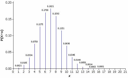
Binomial (n=21, p = 1/3) distribution.
The p-value of this test is P(X>12)
assuming p = 1/3, which can be found by
summing the binomial probabilities for 12, 13, …, 21 successes:  . This p-value can
also be found from the relationship P(X>12) = 1-P(X<11).
Using Minitab’s cumulative distribution function gives:
. This p-value can
also be found from the relationship P(X>12) = 1-P(X<11).
Using Minitab’s cumulative distribution function gives:
Binomial with n = 21 and p = 0.333333
x P( X <= x )
11 0.978806
and so the p-value is P(X>12) = 1-P(X<11) = 1-.9788 = .0212.
This p-value reveals that if the students were just guessing, there’s only about a 2% chance of getting 12 or more correct identifications among 21 trials. In other words, if we repeated this study over and over, and if students were just guessing each time, then a result this favorable would occur in only about 2% of the studies. Since this probability is quite small, we have fairly strong evidence that these students’ process in fact does better than guessing in discriminating among the colas (i.e., that p>1/3). Because the sodas were randomly placed in the cups and (presumably) the teacher kept other variables (e.g., temperature, age) constant, this study attempted to isolate the taste and appearance of the sodas as the sole reasons for their selection.
(b) Yes, the p-value is less than .05, so with that significance level, the teacher would be convinced that his students do better than guessing in discriminating among the colas.
(c) However, he would not have been convinced if his significance level had been .01 since the p-value (.0212) is larger than .01. With the .01 level of significance, it would take 13 successful identifications to convince the teacher, because P(X>13) = 1-P(X<12) = 1-.9932 = .0068, and this is the smallest value of x for which the p-value is below .01. With a significance level of .001, it takes 15 successes to be convincing, because P(X>14) = .0018 is not less than .01, but P(X>15) = .0004 is less than .001.
(d) A Type I error would mean that these students are actually just guessing, but we erroneously conclude that they do better than guessing. A Type II error would mean that the students are not just guessing, but we do not consider the evidence strong enough to conclude that. The p-value of .0212 calculated in (a) is the probability of a Type I error.
(e) Using the .05 significance level, we would reject the
null hypothesis whenever we find 12 or more successes. This is because P(X>12)
= .0212 is less than .05 but P(X>11) = .0557 is not less than
.05. The power of the test at a specific value pa
is the probability of rejecting the null hypothesis when p is actually equal to pa. If we let Y represent
the binomial distribution with n=21 and probability of success pa, then we want to know P(Y>12),
that is, how often will we reject the null hypothesis for when pa is the actual probability of
success. The power of the test can be expressed as: P(Y>12)= ![]() .
.
When the success probability actually equals p=.5, the power is P(Y>12) = 1-P(Y<11) = 1-.6682 = .3318. This can be visualized in the figure below, which displays binomial distributions with p=1/3 and with p=.5.
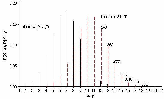
Figure 2: The binomial (21, 1/3) and binomial (21, .5) distributions.
This says that even if students would correctly identify the “odd” cola 50% of the time in the long run, this test only has a 33.18% chance of rejecting the null hypothesis that students are guessing (at the 5% level of significance). So, if the teacher suspected that the success rate might actually be 50%, he should have realized that this study only had about a 1/3 chance of revealing that students do better than guessing
When the success probability actually equals p=2/3, the power is P(Y>12) = 1-P(Y<11) = 1-.1248 = .8752. The next figure displays binomial distributions for this situation, when p=1/3 and when p =2/3.
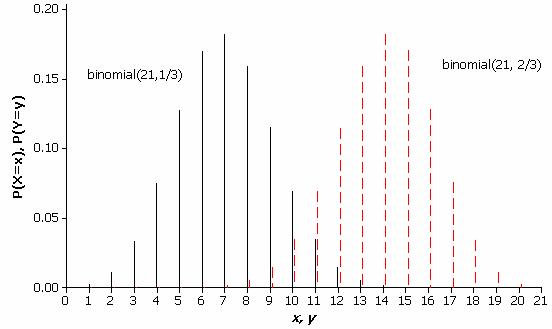
Figure 3: The binomial (21, 1/3) and binomial (21, 2/3) distributions.
This says that if these students would correctly identify the “odd” cola 2/3 of the time in the long run, then this test has an 87.52% chance of rejecting the null hypothesis that the students are guessing. This power is much larger than when p=.5, because the success probability is assumed to be much larger than 1/3 rather than slightly larger than 1/3.
(f) If the teacher wanted the test to be more powerful (statistically), he could have used a larger sample size. Taking a large enough sample would increase the test’s ability to detect that students do better than guessing, even if the actual success probability is not substantially greater than 1/3.
(g) Minitab reports a 95% binomial confidence interval based on these data (12 successes in 21 trials) to be: (.340, .782). The parameter is the probability that a these students correctly identify the odd cola, which is also the long-run proportion of times that these students would make a correct identification. This interval says that it’s plausible that the success probability could be anywhere from .34 to .78. Note that this interval lies entirely above 1/3, which is the success probability if the students are guessing. This concurs with our test of significance in (a) where we rejected 1/3 as a plausible value of p based on how the students performed. In fact, this confidence interval specifies all the plausible values of p that would lead to a two-sided p-value of at least .05.