Example 4.2: Pushing
On
As in many states,
A histogram and summary statistics of the sample data are
below:
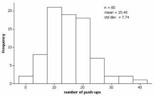
(a) Describe the distribution of the results in this sample.
(b) Suppose we take random samples of 80 males from a very large population. According to the Central Limit Theorem, what can you say about the behavior of the sampling distribution of the sample means calculated from these samples?
(c) If this were a random sample
from a population, would the sample data provide strong evidence that the
population mean differs from 20 push-ups?
Conduct a significance test to address this question. Also calculate confidence intervals to
estimate the population mean with various levels of confidence.
(d) What precautions should we have in analyzing these results?
(e) Would it be reasonable to use this sample to calculate a
prediction interval for the number of push-ups by a 7th grade male
in
Analysis:
(a) The sample distribution has a slight skew to the
right. The average number of push-ups by
the 80 males in the sample was 15.49, with standard deviation 7.74 push-ups. Most students completed about 10-25 push-ups,
with the maximum around 40 or so.
(b) Since the sample size is large (80 > 30), the
sampling distribution of sample means should be approximately normal,
regardless of the population shape, with mean m,
and standard deviation equal to s/![]() . The exact values of m (the population mean number of push-ups
done by 7th grade males) and s
(the population standard deviation) are unknown, but they should be in the ball
park of 15.49 and 7.74, the sample statistics.
. The exact values of m (the population mean number of push-ups
done by 7th grade males) and s
(the population standard deviation) are unknown, but they should be in the ball
park of 15.49 and 7.74, the sample statistics.
(c) Test of significance: If this was a random sample from a larger population of 7th graders, let m represent the mean number of push-ups that would be completed in this population. We want to decide whether m is significantly different from 20.
H0: m = 20 (the population mean number of push-ups is 20)
Ha; m ≠ 20 (the population mean differs from 20)
Since we are working with a quantitative response variable and
the sample size is large, we will model the sampling distribution of the sample
means with the t distribution with
80-1=79 degrees of freedom.
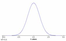
![]() =-5.21
=-5.21
p-value = 2P(T79 <-5.21) = 2(.0000007) = .0000014
Student's
t distribution with 79 DF
x P( X <= x )
-5.21 0.0000007
With such a small p-value, we easily reject the null
hypothesis and conclude that the population mean
number of push-ups differs from 20. While
the test tells us that the sample data provide overwhelmingly strong evidence
that the population mean is not 20, it does not tell us what values are in fact
plausible for the population mean.
Confidence Intervals:
Again let m represent the mean number of push-ups that would be completed in the hypothetical population of 7th graders.
Since we are working with a quantitative response variable and the sample size is large, we will model the sampling distribution of the sample means with the t distribution with 80-1=79 degrees of freedom.
To construct a 95% confidence interval for m, we will use t*79=1.990
Inverse
Cumulative Distribution Function
Student's
t distribution with 79 DF
P( X <= x ) x
0.025 -1.99045
![]() = 15.49 + 1.72 = (13.76,
17.21)
= 15.49 + 1.72 = (13.76,
17.21)
Verifying these calculations in Minitab, we would find:
Test
of mu = 20 vs not = 20
N Mean StDev SE Mean 95% CI T P
80 15.4900 7.7400
0.8654 (13.7675, 17.2125) -5.21
0.000
Based on this sample, assuming it represents the larger
population, we are 95% confident that the average number of push-ups completed
by all 7th graders in the population is between 13.76 and 17.21, so
20 is rejected as a plausible value at the .05 level of significance. We could also find 99% and 99.9% confidence
intervals for m to be:
95%: ![]() = 15.49 + 2.28 = (13.21, 17.77)
= 15.49 + 2.28 = (13.21, 17.77)
99%: ![]() = 15.49 + 2.96 = (12.53, 18.45)
= 15.49 + 2.96 = (12.53, 18.45)
Thus, even with these stricter standards of 99% and 99.9%
confidence, we still have reason to believe that the population mean is less
than 20 push-ups. These results are
consistent with the extremely small p-value from the significance test above.
(d) We should be very cautious in generalizing these results
as we don’t know if the push-up performance of the students sampled at this
rural high school in
(e) If we wanted to calculate a prediction interval, we would have the same concern that this sample may not be representative of 7th graders across the state, and the additional concern that the population distribution may not follow a normal distribution. We have reason to doubt that it does since the sample shows some skewness to the right. So while we may want to predict the number of push-ups by an individual in this population, it would be risky to do so with these data.