Stat 414 – Review I

(Draft 2 10/18)

Participation credit (preferably before Tuesday, 8am): In Canvas,

(1) post at least one question you have on the material described below.

(2) post at least one example question that you think I could ask on the material described below

Optional Review Session: Tuesday 5-6pm (zoom) ?

Optional Review Problems: review1probs.html

Format of Exam: The exam will cover Lectures 1–9, Quizzes 1-8, Computer problems 1-8, Homeworks 1-4.  There will be a “written” component and a “computer” component. The two components will be designed to take 75 minutes. The exam will be worth approximately 75 points.

· For the written component, you should expect me to provide output and focus on interpretation of the models and concepts.  Be ready to explain your reasoning, including in “laymen’s” language, as well as to write model equations and interpret variance-covariance matrices. You may use one 8.5 x 11 page of notes (hard copy).

· For the computer component, you will be expected to access a data set and answer questions about it.  (So for example, I could ask you to calculate an ICC from output or using the computer after you decide what model to run.)  This portion is open notes. All reference material should come from this course only.

Advice: Prepare as if a closed-book exam. Review Quizzes/commentary, HW solutions/ commentary, Lecture notes (annotated files). The first exam is really all about components of regression models: model assumptions, residual plots (standardized residuals), model equations ( vs. , ordinary least squares vs. generalized least squares vs. maximum likelihood estimation, slope vs. intercept, Residual error (MSE, SE residuals), Indicator vs. Effect coding, Centering, Adjusted vs. Unadjusted associations, Within vs. Between group associations, Random vs. Fixed Effects.  This means you have learned about “basic mixed models” but I might still wait before reading those specific materials.

Italics indicate related material that may not have been explicitly stated in this course but you are still responsible for knowing.

What you should recall from previous statistics courses

· Mean = average value, SD = typical deviation in data from average value

· The basic regression model, Y_i =  + x_i,

o  represents the part of the response (dependent) variable that cannot be explained by the linear function.

o Matrix form

§  measures the unexplained variability of the responses about the regression model

o Least squares (OLS) estimation minimizes SSError =

§  (p = number of slopes)

§

o Use output to write a fitted regression model using good statistical notation

o Interpreting regression coefficients in context

§  = expected vs. predicted mean response when all x = 0

· But often extrapolating unless the explanatory variable(s) have been centered

§  = expected vs. predicted change in mean response for x vs. x + 1

o The difference between the model equation (e.g., E(Y) = ) and the prediction equation (e.g.,

o Checking model assumptions

§ Residuals vs. Fits should show no pattern to satisfy Linearity (E(Y) vs. x)

§ Errors should be Independent,

§ (Conditional) residuals should look roughly Normal (Y | x ~ Normal)

§ Residuals vs. Fits should show no fanning or unequal spread to satisfy Equal variance

· Var(Y | x) is the same at each value of x

o aka heteroscedasticity vs. homoscedasticity

§ Violation of model assumptions usually leads to bad estimates of

· Usually underestimating (overstating significance)

o Also assuming x values are fixed and measured without random error

o Also assuming you have the “right” variables in the model

o Unusual observations can be very interesting to explore

§ High leverage: observation is far from center of x-space

§ Influential: removal of observation substantially changes regression model (e.g. Cook’s distance explores change in fitted values)

· Combination of high leverage and/or large residual

· Use individual t-statistic or F-statistic to judge significance of association (slope coefficients)

o t-statistic is adjusted for all other variables in the model (two-sided p-values assuming the variable was the last one entered into the model)

§ Values larger than 2 are generally significant

§ For individual terms, generally t = (estimate – 0)/SE(estimate)

o “overall F-test” tests all slopes are zero (compares full model to model with only intercept) vs. at least one slope differs from zero

o “partial F-test” tests some slopes are zero (compares full model to reduced model)

§ especially helpful for categorical variables or after adjusting for a specific subset of variables

· Analysis of Variance (ANOVA)

o Traditionally thought of as method for comparing population means but more generally is an accounting system for partitioning of variability of response into model and error

o To compare groups, assume equal variances

§ s_p = residual standard error = root mean square error = “pooled standard deviation”

o SSTotal =  == SSModel + SSError  with df = n – 1

o F = MSGroups / MSError (Between group variation / Within group variation)

§ Values larger than 4 are generally significant

§ When just two groups is equivalent to a pooled two-sample t-test

· R² = percentage of variation in response explained by the model

o 1 – SSError/SSTotal  1 –

o

o Explain similarities and differences in how R² and R²_adj are calculated (whether or not adjust for df)

· Changes that you expect to see when you make modifications to the model, e.g., adding a variable

o Explain that adding terms to the multiple regression model “costs a df” for each estimated coefficient and reduces df error

o If the new variable is “orthogonal” to current variables, coefficients won’t change but SSError will (hopefully) decrease

o If the new variable is related to current variables, “adjusted associations” can look very different from unadjusted associations

§ Interpreting coefficients MUST account for the other variables in the model

o Advantages/Disadvantages to treating a variable as quantitative or categorical

§ Recognizing which R has done and when might be appropriate

· Using MSError and R² to evaluate a model performance

o Slight differences in interpretation (e.g., typical prediction error vs. comparison to original amount of variation in response)

o Comparing models

· Explain that least squares estimates are unbiased for regression coefficients (and how we decide)

From Day 1 you should know how to

· Identify whether a study plan is likely to result in correlated observations

o e.g., repeat observations, clustered data, cluster-randomized trials

· Interpret sample standard deviation (even for a “no variable model”) as “typical prediction error”

· Fitting and interpreting a linear model with no predictors (e.g., a “null model”)

· Using R² as a measure of percentage of reduction in SSError compared to the null model

· What is measured by

From Quiz 1

· Distinguishing Level 1 and Level 2, as well as variables measured at Level 1 vs Level 2

From Computer Problem 1

· How sampling plan can impact standard error, especially cluster sampling

From Day 2 you should know how to

· Explain that “least squares regression” (OLS) and minimizing the sum of squared residuals is just one possible method for fitting a model

o Explain the relationship between residual standard error and MSError

· Interpret intercept and slope coefficients in context

o Advantages of using something other than a “one unit” increase depending on scaling/context

· Define and evaluate the basic regression model assumptions (LINE) for inference with least squares regression (in context)

o Can also use residual plots to check for patterns/relationships

· Explain how  measures sample to sample variation in  values from different random samples

o Explain that  depends on , n and SD(X).

§  for multiple regression; simplifies to  for simple regression (1 EV)

§ In multiple regression, also depends on the linear correlation among predictor variables (“variance inflation factor”)

· Explain that maximum likelihood estimation is another method for fitting a model that focuses on maximizing the ‘likelihood’ of obtaining the observed data

o Estimates of coefficients usually match but can change estimates of variability (e.g., residual standard error)

o (Day 3) REML estimates variance terms slightly different and usually looks more like OLS

o When sample sizes are large there aren’t major differences among the three estimation methods

o Be able to identify which method is being used by the software

· Identify AIC and BIC as alternative “measures of fit” (balance between achieved likelihood and complexity of the model (df)) and can be used to compare models

· Determine the df used by a model

o OLS vs. ML/REML

o Including whether use additional variance terms in the model (e.g.,  per month)

From Quiz 2

· Interpreting the model (e.g., slope vs. intercept vs. residual)

· Interpreting the form of the model, both visually and via model equation

· What influences , the accuracy of our estimate of a slope coefficient

· Reading residual plot

From Computer Problem 2

· Evaluating LNE using residual plots

From HW 1

· Defining meaningful variables for a given context (e.g. time vs. speed vs. adjusting for track length)

· Suggest possible remedies for violations of basic model assumptions

o Transformations of y and/or x can improve linearity

o Transformations of y can improve normality and equal variance

o Including polynomial terms can model curvature

· Contrast the behavior between a log transformation and a polynomial model

· Understand impacts of centering a variable on interpretation, significance of model

· Identify benefits of centering a variable

o Interpretation of intercept

o Reduce multicollinearity of “product” terms (e.g., x and x²)

· Visually comparing graphs of the data to models, smoothers

o Don’t call all models “lines”

· Define multicollinearity and its consequences

o explanatory variables have a strong linear association

· Use VIF values to measure amount of multicollinearity in a model

o VIF = variance inflation factor, measures R² from regressing one explanatory variable on all the others

o Variables with high VIF will have inflated standard errors/misleading information about significance of the variable in the model

o Usually VIF values larger than 5 or 10 are concerning

o Remedies include reexpressing variables, removing variables, centering (some cases)

· Standardizing can also make regression coefficients more comparable by putting the variables on the same SD scale

From Day 3 you should know how to

· Set up and carry out a test of significance for a population slope

o Including stating the null and alternative hypotheses both in symbols and in words

· Describe and interpret properties of repeated random samples and fitting regression lines

· Carry out and interpret the t statistic and the F statistic; interpret p-value as a measure of “strength of evidence” against the null hypothesis

· Carry out a Likelihood Ratio Test (LRT) to compare nested models

o Difference in log likelihood values (x2)

o Compare to chi-square distribution with df = difference in number of parameters between the two models

· Consider whether one model is “nested” in another

o Can you get from one model to the other by setting some of the parameters to 0?

o Can sometimes still get a “rough comparison” of not-nested models

From Quiz 3

· Counting number of parameters (df) used by a model

o When counting parameters, REML/ML count the parameter, OLS does not

o Remember the slope is the “parameter,” not the variable

· Interpreting the confidence interval for a slope

· The relationship between residual standard error and MSE

From Computer Problem 3

· Confidence interval for mean response vs. Prediction interval for future value.

· Properties (e.g., curvature) of confidence and prediction bands

· short-cut for prediction intervals

· Watch for “hidden extrapolation”

From Day 4, you should be able to

· Interpret R’s Scale-Location plot as a measure of heteroscedasticity

o A linear association in this graph suggests a trend in the magnitude of the residuals vs. the fitted values

o Some methods (e.g., Bruesch-Pagan Test) provide a p-value for the strength of evidence of a linear association between the absolute residuals and x.

· Explain the principle of weighted least squares to address heteroscedasticity in residuals

o

o Giving less weight in the estimation of the “best fit” line to observations that are measured with more uncertainty

o Use standardized residuals in residual plots to evaluate the appropriateness of the model

o Predict how the fitted model will change when weights are applied

o Predict how prediction intervals will change

· Evaluate other remedies for heteroscedasticity including

o Transforming the response variable

o Estimating the variances terms from the residuals (e.g., HC standard errors)

§ Explain the idea of “sandwich estimators” for “correcting” the standard errors of the coefficients when heteroscedasticity is present

§ HC corrected standard errors are another way to “fix” the standard errors in the presence of heteroscedasticity. This again is like using the observed variance estimates to tweak the matrix that computes the standard errors.

o Modelling a more complicated variance-covariance matrix (generalized least squares)

§ WLS is a special case

§ Can often use LRTs to compare model performance

§ Remember to use standardized residuals to assess the equal variance assumption with weighted LS

· Keep in mind that  is about the variation in the residuals after accounting for the model

From Computer Problem 4

· Be able to use the output to reconstruct components of the variance-covariance matrix of the errors

· Count parameters

· Use likelihood ratio test to compare models

· Compare model behavior to observed data

From Quiz 4

· Predicting how a weighted regression model might differ from the unweighted model based on which observations receive more/less weight

· Understanding the fixed vs. random terms in our model equation

· Distinguishing between what R² measures and what residual standard error measures

· Notation

o If start with E(Y) then “error term” is not there

o E(Y) represents the “expected” or “true population mean” response

o  is the predicted response and the predicted population mean

From HW 2

· Utilize residual plots to evaluate validity conditions

o Identify which plot to use and what you learn from the plot

o Also review study design (independence)

· Understand how different weighted regression models estimate variances

o e.g., given the model output, calculate the estimated variance

o Evaluate (differently) “significant improvement in model fit” and “improving the validity of the model”

· Pros and Cons of variable-transformations

o Only transforming y will impact “distributional assumptions”

o Transforming only one variable impacts only that variable’s linear relationship with y (e.g., if all relationships are nonlinear vs. just one)

o Explain that transformations may not be able to “solve” more complicated unequal variance patterns

§ Consider whether Var(Y) is changing with an explanatory variable (e.g., increasing variability with larger values of x)

§ Explain the principle of obtaining an estimate of  when have unequal variance

· e.g., Var(Y_i

· This can impact judgement of significance of terms in model, predictions, etc.

· Distinguish between a confidence interval for E(Y) and a prediction interval for y

o Population regression line vs. variability about the line

o Identify a 95% prediction interval for an individual observation as roughly

o What does/does not impact the widths of these intervals

From Day 5, you should be able to

· Identify and interpret all the components of a basic ANOVA table

· Differentiate eta-squared from omega-squared vs. ICC

· Be able to calculate and interpret an ANOVA ICC from the ANOVA table

· Add a categorical variable to a regression model using k – 1 terms for a variable with k categories

o  where  is the k^th “group effect”

o Indicator variables change intercepts

o Interpret coefficients as changes in intercepts (e.g., parallel lines, at any value of x)

· Use either effect coding or indicator coding

o Determine the value of the coefficient not displayed in the output

o Interpret signs of coefficients (comparing to overall mean or to reference group)

o Interpretation of intercept (reference group vs. overall mean)

· Explain and evaluate model assumptions (normality, equal variance) with categorical data

· Carry out test of significance involving individual or groups of slope coefficients

o Stating appropriate hypotheses for removing the variable

o Use a “partial F-test” to test significance of categorical variable or a subset of variables

§ Null is all k-1 coefficients are zero; Alt. is at least one coefficient differs from 0

§ Compares increase in SSError with the reduced model to MSE for the full model to is see whether reduced model is significantly worse (df num = k – 1, df denom = MSE df for full model)

o Special cases of partial F tests:

§ One coefficient (equivalent to t-test as last variable entered into model)

§ All coefficients (“model utility test”)

o Use “anova(model1, model2)” to carry out partial F-test in R.

From Quiz 5

· Effect (contr.sum aka “sum to zero”) vs. Indicator coding (contr.treatment)

o Seeing this in the code is one way to know which way the variables have been coded

· Interpreting slopes and intercepts with categorical variables

From Computer Problem 5

· The distinction between  and

· Check degrees of freedom used when including categorical variables

· Interpreting the model (effect coding and indicator coding)

From Day 6, you should be able to

· Interpret an added-variable plot (residuals of y on x₁, … x_p vs. residuals of x_p+1 on x₁, … x_p to understand whether x_p should be added to the model and in what form

· Interpret the nature of the adjusted association

o From graph

o From multiple regression model

· Interpret intercept and slope coefficients for multiple regression model in context

o Multiple regression: After adjusting for other variables in the model (e.g., comparing individuals in the same sub-population)

§ Effect of x₁ on y can differ when x₂ is in the model

§ Adjusted and Unadjusted relationships can look very different

o Identify the other variables you are talking about

o Quotes: We interpret the regression slopes as comparisons of individuals that differ in one predictor while being at the same levels of the other predictors. In some settings, one can also imagine manipulating the predictors to change some or hold others constant—but such an interpretation is not necessary. This becomes clearer when we consider situations in which it is logically impossible to change the value of one predictor while keeping the value of another constant (e.g., x and x²).  A better interpretation is that beta1-hat is "the change in Y when X1 changes by one unit, allowing for simultaneous linear change in the other predictors” or, alternatively, …after removing the linear effects of the other x’s from both y and  x1

o Bottom line: make sure you can make sense of the phrase “after adjusting for…”

· Distinguish the meaning of sequential vs. adjusted sums of squares

· Interpret the ICC as a measure of correlation between two responses within the same group

From Quiz 6

· Adjusted associations can be very different from unadjusted associations

· The  for a model with two variables could be smaller than the sum of the  values from the one-variable models if the predictor variables explain some of the same variability in the response

· Between group variation vs. within group variation

From Computer problem 6

· Connection between  and  for a categorical variable

· Using R to calculate ICC

From HW 3

· Interpreting coefficients in a model regression model

· Within vs. Between group associations

o Aggregating vs Disaggregating data

o Adjusting for level 2 grouping variable

o Group mean centering vs. grand mean centering

o Between group regression focuses on the association between  and , the group means

o The within group regression focuses on the association between  and  within each group, assuming it’s the same within each group

o The between group regression slope may look very different (even opposite in direction) from the within group regression slope

o Regular regression can be written as a combination of the within and between group regressions, e.g.,

§  matches the within group regression coefficient

§  is the between group coefficient minus within group coefficient (so the difference between them)

§ Using a “deviation variable” instead: regressions, e.g.,  actually separates the within group () and between group () components.

· Compute the effective sample size of a study based on the ICC, (common) group size, number of groups

o Compromise between group size and number of groups

From Day 7, you should be able to

· Use generalized least squares to add a correlation parameter to an OLS model to model within group correlation

· Understand how this impacts the variance-covariance matrix

· Interpret values in the estimated variance-covariance matrix

· Understand how this impacts the standard error of certain parameter estimates (intercept, group differences)

· Translate between covariances and correlations

From Computer problem 7

§ Adding a categorical variable into the model may be enough to account for intraclass correlation

§ This often impacts standard errors of other variable coefficients, e.g., reducing the effective sample size of a  estimate

§ Bottom line: If you have correlated/clustered observations, your “naïve” standard errors are likely too small, overstating significance

From Quiz 7

§ Recognizing effect vs. indicator coding

§ How the relationship between x1 and x2 impacts the relationship between y and x1 when x2 is added to the model (adjusted vs. unadjusted associations)

From Day 8, you should be able to

· Explain the basic principles behind treating a factor as “random effects” rather than “fixed effects”

§ Identify some benefits of random effects models

· Degrees of freedom

· Observed “levels” are representative of a larger population (random sample?)

· Want to make inferences to the larger population

· [Later: Use of Level 2 units + Level 2 variables in same model]

· Compute the ICC in terms of random effects (between group vs. total variation)

§ Standard errors reflect the randomness at the individual level and from the random effect (e.g., sampling error)

· Fit and interpret the “random intercepts” model

o Like adding the “grouping variable” to the model but treating as random effects

o “may be all that is required to adequately account for the nested nature of the grouped data.”

o “there is virtually no downside to estimating mixed-effect models even when If is small or non-significant because in these cases the mixed-effect models just return the OLS estimates” (Bliese et al., 2018)     

o Also known as “unconditional means” or “null” model or “one-way random effects ANOVA” (assumes equal group sizes)

· Explain the principle of shrinkage/pooling as it pertains to multilevel models

o  where

o No pooling « weights = 1 (treating as fixed effects)

o Complete pooling « weights = 0 (no group to group variation)

o Identify and explain factors that impact the size of the weights/consequences/amount of shrinkage

o Determine when an estimated mean will be closer to the group mean vs. the overall mean

· Write out the random intercepts model:  where

o

· Interpret R output (lme, lmer)

o How to use nlme::lme and lme4::lmer in R

o Is output reporting  or ?

· Discuss consequences of treating a factor as random effects

o Impact on model equations (now estimating one parameter = )

o Total Var(Y) = +

o ICC =

o Variance-Covariance matrix for the observations

o Impact on standard errors of coefficients (adjusting for dependence)

· Compute and interpret intraclass correlation coefficient as expected correlation between two randomly selected individuals from the same group

o Show how this correlation coefficient is “induced” by using the random intercepts model

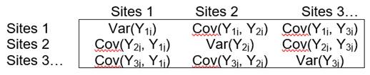
· Be able to explain/interpret the variance-covariance matrix for the responses

Covariance

	Site 1 (beach 1)	Site 2 (beach 1)	Site 3 (beach 2)	Site 4 (beach 2)
Site 1 (beach 1)			0	0
Site 2 (beach 1)				0
Site 3 (beach 2)
Site 4 (beach 2)	0	0

Correlation

	Site 1 (beach 1)	Site 2 (beach 1)	Site 3 (beach 2)	Site 4 (beach 2)
Site 1 (beach 1)			0	0
Site 2 (beach 1)			0	0
Site 3 (beach 2)	0	0
Site 4 (beach 2)	0	0		1

From Quiz 8

· Think of the Level 2 units as a sample from a larger population with variance

· Using the normal distribution to predict other judges

· Understanding how individual effects are calculated and what factors impact the precision of those estimates (formula for )

· Q5 (e):  Want to estimate  (and I’m hand-waving this vs. )

o  is what I would use if all I had were 5 observations

o  is what I use if I am assuming equal variances across groups and what to use the pooled standard deviation as the residual standard error

o  is what I use with a mixed effect model (again, pooling across groups, taking group size into account, but with shrinkage)

From Quiz 8/Computer Problem 8

· Understanding the “weights” used in “partial pooling” and what makes them larger/smaller and how this changes the estimate of the group mean (between observed group mean and ‘overall’ mean)

· Reminder: If adding/removing a variable from the model changes other coefficients, then that variable is related to other variables in the model (not orthogonal)

From HW 4

· Distinguish between different models (e.g., individual vs. aggregated data, whether or not assuming/have independent groups)

· Shrinkage; complete pooling vs. no pooling vs. partial pooling

· Identifying different “variance components”

· Again, within group vs. between group association, including Level 2 group means in the model, with and without the deviation variable

From Day 9

· Assess the statistical significance of the variation among Level 2 units

o Stating null and alternative hypotheses

o Fixed effects ANOVA

o Confidence intervals for variance components

o Likelihood ratio test (MLE or REML approach)

§ Cut p-value in half?

· Understand that we don’t normally make the fixed vs. random decision based on a likelihood ratio test, but instead consider the study design/research question of interest

· Identify Level 1 and Level 2 from study design/research question

· Write out the statistical model for a “random intercepts” model (’s, u_j, s, )

o Interpret model components

o Define indices

o Interpretation of intercept

o Standard deviations vs. variances vs. covariances

o Composite equation vs. Two-level equations

· Identify number of units at each level

· Add a Level 1 variable to the random intercepts model

o Interpretation of “adjusted” association, parameter estimates

§ Also remember to zero out (intercept) or “fix” Level 2 units (e.g., for a particular school)

o Visualize the model (e.g., parallel lines)

o Level 1 and Level 2 equations, composite equation

o R² type calculations

o Assessing significance (t-test vs. likelihood ratio test)

· Explain the distinction between variation explained by fixed effects vs. by random effects

· Explain the distinction between total variation and variation explained by random effects after adjusting for fixed effects

· Calculate percentage change in Level 1, Level 2, and overall variation after including variable

· If a variable coming into the model is related to the level 2 units, variation explained will depend on the nature of that relationship (similar to adjusted associations in regular regression models)

· Include a Level 1 variable and reinterpret coefficients, variance components as adjusted for that variable

§ Also remember to zero out (intercept) or “fix” Level 2 units (e.g., for a particular school)

Keeping track of variances

·  = variation in response variable

·  = standard deviation of explanatory (aka predictor) variable

·  = variation about regression line/unexplained variation in regression model, variation in response at a particular x value

o  aka s aka s_e = residual standard error = square of sum of squared residuals (“root MSE”)

·  = sample to sample variation in regression coefficient

·  = sample to sample variation in estimated predicted value.  There are actually two “se fit” values, one for a confidence interval to predict E(Y) and one for a prediction interval to predict . The latter can be approximated with , but actually depends on  etc.