Stat 414 - Review 1 Problems
The following are previous exam problems and application problems. The exam this quarter will also involve some more "conceptual" problems as you have been seeing on the quizzes. I also expect interpretation of output I provide. You should assume all of the questions below have "Explain"after them.
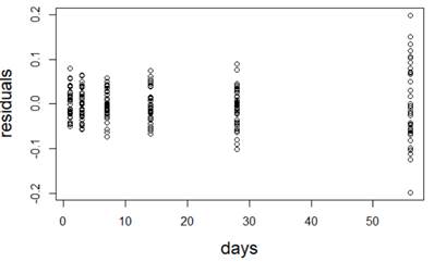
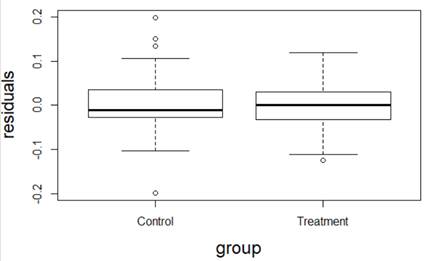
(a) I have fit a rather complicated single-level nonlinear model to these data (using days and group as explanatory variables). Assess the validity of my model. Be very clear how you are evaluating each assumption:
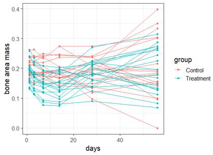
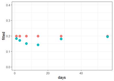
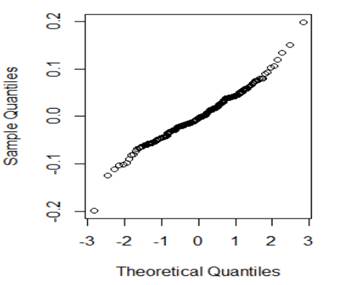
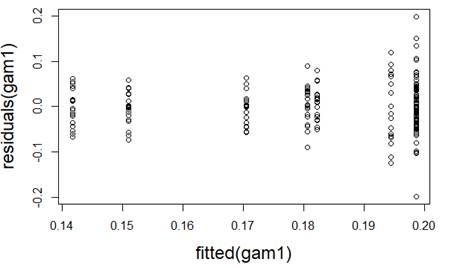
(b) Which of the following would you consider doing next to improve the validity of the model? Briefly justify your choice(s).
Transformation to improve linearity
Quadratic model to improve linearity
Transformation of response to improve normality
Transformation of explanatory to improve normality
Include days in a weighted regression
Include group in a weighted regression
Multilevel model using mouse as a grouping variable (Level 2 units)
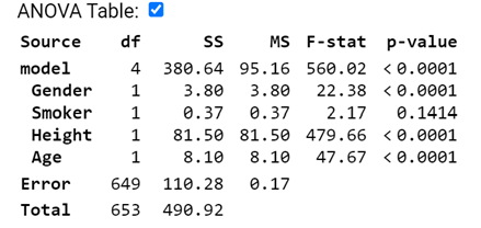
2) Data were collected on 654 youths in the area of East Boston during the middle to late 1970s. The youth in the study were of ages 3 to 19 years, an age period during which much physical development, such as increase in lung capacity, takes place. The objective was to analyze the relationship between smoking status, and forced expiratory volume (FEV, measured in liters). (FEV is a measure of strength of a persons lungs the maximum volume of air a person can blow out in the first second; higher numbers are better/healthier lungs)
Consider the following model
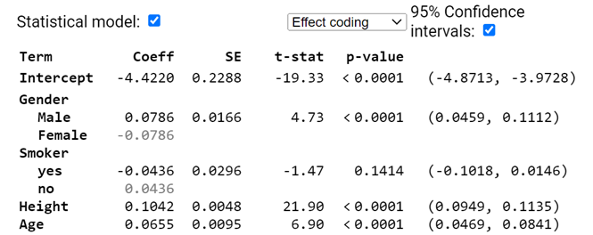
(a) Provide a rough estimate of a 95% confidence interval for a 17-year-old male smoker who is 64 inches tall.
(b) Interpret the (0.0459, 0.1112) interval in context.
(c) Smoker doesnt appear to be significant in this model. Explain two distinct ways I can tell this?
(d) Would it be reasonable to conclude the smoking status is not related to FEV?
(e) State the null and alternative hypotheses for removing Smoker from the model. Is the p-value for this test in the above output?
(f) If I remove the height variable, smoker is now significant at the 5% level. What does this tell you?
3) Recall our Squid data
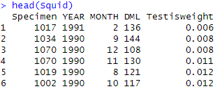
Squid$fMONTH
=
factor(Squid$MONTH)
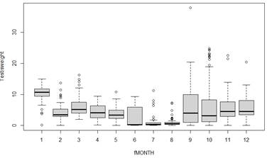
plot(Testisweight ~ fMONTH, data=Squid)
The graph below shows the predicted values for each month (along with standard errors).
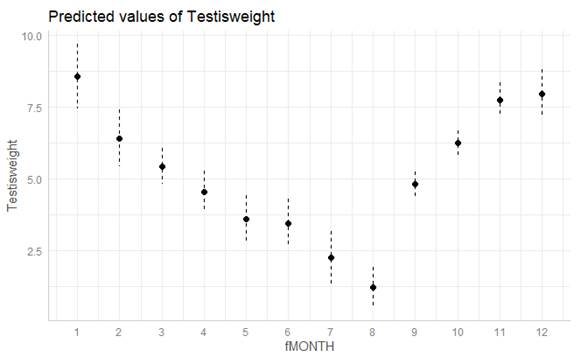
(a) If this model was fit with indicator coding and fMONTH = 1 as the reference group, is the coefficient of fMONTH2 positive or negative?
(b) If this model was fit with effect coding, is the coefficient of fMONTH2 positive or negative?
(c) Continuing (b): If fMONTH1 is the missing category, will its coefficient be positive or negative?
Suppose
we use
the sample variance for each month as an estimate for ![]()
(d) Which months do we want to 'downweight' in estimating the model?
(e) Conjecture what changes you would expect to see in the previous graph in this weighted regression model.
(f) How do you expect the residual standard error to change in the weighted regression model?
price = price for one night (in dollars)
overall_satisfaction = rating on a 0-5 scale
room_type = Entire home/apt, Private room, or Shared room
TransitScore = quality of the neighborhood for public transit (0-100)
neighborhood = neighborhood where unit is located (1 of 43)
(a) Identify the Level 1 units and the Level 2 units.
Consider the following partial output for the multilevel model (Indicator parameterization was used for room size)
Fixed effects:
Estimate Std. Error t value
(Intercept) 25.353 26.454 0.958
overall_satisfaction 24.919 5.508 4.524
room_typePrivateroom -82.739 3.831 -21.598
room_typeSharedroom -105.875 10.960 -9.660
Number of Observations: 1561
Number of Groups: 43
Analysis of Variance Table
npar Sum Sq Mean Sq F value
room_type 2 2525146 1262573 244.195
overall_satisfaction 1 105350 105350 20.376
(b) Conceptually which
do you expect
to be larger  or
or  ? Explain your
reasoning.
? Explain your
reasoning.
(c) Interpret the intercept coefficient in context.
(d) Interpret the coefficient of overall_satisfaction in context.
(f) Consider the following two variables:
- PctBlack = proportion of black residents in a neighborhood
- HighBlack = 1 if PctBlack above .60, 0 otherwise
Explain why you might choose to use the second variable rather than the first variable in the model. Do you expect the coefficient of HighBlack to be positive or negative? Explain your reasoning.
(g) Consider the first few observations of the first row of the 1561 x 1561 variance-covariance matrix for the above model output
![]()
Where will the first non-zero value occur?
(h) Here is the first row of the corresponding correlation matrix
![]()
Verify the value for 0.0861.
(i) If I were to look at the first row of the corresponding correlation matrix for the null model, how do you think the second value will compare? (likely) Explain your reasoning.
5) Consider the following two models for predicting language scores for 9 different schools. IQ_verb is the students performance on a test of verbal IQ.
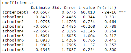
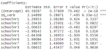
Which model demonstrates more school-to-school variability in language scores?
6) Give a short rule in your own words describing when an interpretation of an estimated coefficient should hold constant another covariate or set to 0 that covariate
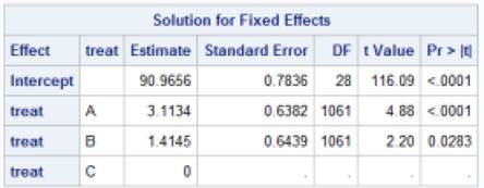
7) The following SAS output is from modeling results for a randomized controlled trial at 29 clinical centers. The response variable is diastolic blood pressure.
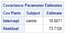
(a) What is the patient level variance? (Clarify any assumptions you are making about the output/any clues you have.)
(b) What is the center level variance?
(c) What is an estimate of the ICC? Calculate and interpret.
(d) What is the expected diastolic blood pressure for a randomly selected patient receiving treatment C at a center with average aggregate blood pressure scores?
(e) What is the expected diastolic blood pressure for a randomly selected patient receiving treatment A at a center with aggregated blood pressure scores at the median?
(f) What is the expected diastolic blood pressure for a randomly selected patient receiving treatment C at a center with aggregate blood pressure scores at the 16th percentile?
(g) What is the expected diastolic blood pressure for a randomly selected patient receiving treatment B at a center with aggregate blood pressure scores at the 97.5th percentile?
Below are the graphs and output related to regressing the ppvt score on the mother's age
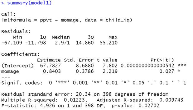
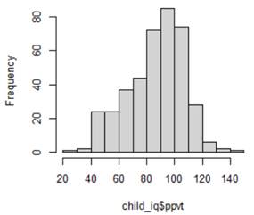
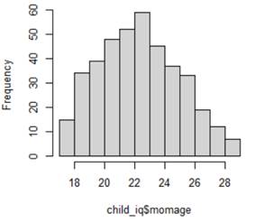
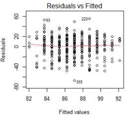
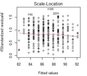
(a) (2 pts) Linearity
(b) (2 pts) Equal variance
(c) (2 pts) Normality
(d) (2 pts) Independence
9) For same dataset, model
(a) (3 pts)
Provide a
one-sentence interpretation of the following output
predict(model4, newdata = data.frame(momage=30), interval = "prediction")
fit lwr upr
1 95.89836 56.38459 135.4121
(b) (2 pts) Suppose instead we used interval = "confidence"
1. Identify one thing that will not change in this output
2. Identify one thing
that will
change in this output