Stat 414 – Final Exam Review Solutions

 

0) Consider this excerpt: “application of multilevel models for clustered data has attractive features: (a) the correction of underestimation of standard errors, (b) the examination of the cross-level interaction, (c) the elimination of concerns about aggregation bias, and (d) the estimation of the variability of coefficients at the cluster level.”

Explain each of these components to a non-statistician.

(a) Assuming independence allows us to think we have a larger sample size (more information) than we really do and underestimates standard errors.

(b) Including interaction terms between Level 1 and Level 2 variables

(c) Still get to analyze the data at Level 1 vs. aggregating the variables to Level 2 which could have a different relationship than the Level 1 relationship. It’s problematic to assume the Level 2 relationship applies to individuals.

(d) We are able to estimate the intercept-to-intercept and slope-to-slope variation at Level 2

 

Consider this paragraph: The multilevel models we have considered up to this point control for clustering, and allow us to quantify the extent of dependency and to investigate whether the effects of level 1 variables vary across these clusters. 

(e) I have underlined 3 components, explain in detail what each of these components means in the multilevel model.

Control for clustering: We have observations that fall into natural groups and we don’t want to treat the observations within the groups as independent, by including the “clustering variable” in the model, the other slope coefficients will be “adjusted” or “controlled” for that clustering variable (whether we treat it as fixed or random)

Quantify the extent of the dependency: The ICC measures how correlated are the observations in the same group

Whether the effects of level 1 variables vary across the clusters: random slopes

 

(f) The multilevel model referenced in the paragraph does not account for “contextual effects.” What is meant by that?

The ability to include Level 2 variables, variables explaining differences among the clusters.  In particular, we can aggregate level one variables to be at Level 2 (e.g., group means). Being able to include these in the model, along with controlling for the individual groups, is another huge advantage of multilevel models.

 

(g) What can you tell me about the assumptions made the following models (Hint: no pooling, partial pooling, complete pooling?)

lm(y ~ 1) This fits one line (and actually just one intercept estimating the overall mean response) and completely ignores any Level 2 units/group/assumes all of the observations are independent. This is “complete pooling.”

lm(y ~ 1 + factor(school_id) This fits “school effects” but treats them as fixed. Each school gets a term in the model using either effect or indicator coding, k -1 parameters are estimated for the schools. This is “no pooling.”

lmer(y ~ 1 + (1 | school_id) This fits “school effects” and treats them as random. The only parameter added to the complete pooling model is , the school-to-school standard deviation in the intercepts.  This is “partial pooling,” as the school estimates will be shrunk together a bit as we assume they are coming from a normal population rather than estimating them all individually.

 

(h) Complete these sentences:

Only  level 1 variation in predictors (aka covariate aka explanatory variable)             can reduce level-1 variance in the outcome

Only level 2 variation in predictors*                               can reduce level-2 variance in the outcome

Only cross-level interactions                       can reduce variance of random slopes

*The subtle reminder here is that “level 1 variables” can have explain variation at both level 1 and level 2 if they vary both within groups and between groups.

 

 

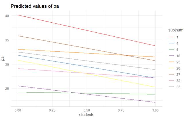
1) Let’s consider some models for predicting the happiness of musicians prior to performances, as measured by the positive affect scale (pa) from the PANAS instrument. MPQ absorption = levels of openness to absorbing sensory and imaginative experiences

 

Model0

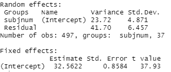
(a) Calculate and interpret the intraclass correlation coefficient

(23.72)/(23.72 + 41.70) = 0.363

36% of the variation in pa scores (pre-performance happiness) is at the musician level (i.e., is attributable to differences among musicians)

And/Or

The correlation between two performances for the same musician

 

Model1

instructor = ifelse(musicians$audience == "Instructor", 1 , 0)

students = ifelse(musicians$audience == "Students", 1, 0)

summary(model1 <- lmer(pa ~ 1 + instructor + students +  (1 + instructor + students | subjnum), data = musicians))

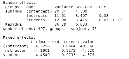
(b) Interpret the 34.73, -4.19, and 4.51 values in context.

34.73: the estimated pre-performance happiness for musicians playing in public or juried recitals (the other two performance types) for the average performer (or estimated population mean)

 

-4.19: The estimated decrease in pre-performance happiness for a particular performer, on average, with an instructor for the audience compared to public or juried recitals

 

4.51: The estimated performer-to-performer population standard deviation in pre-performance happiness for public or juried performances.

 

(c) Calculate a (pseudo) R² for Level 1 for this model.

Comparing the Level 1 variance between Model 0 and Model 1:

1 – 36.39/41.70 = .127

12.7% of the performance to performance pre-performance happiness levels within a performer can be explained by type of audience (instructor, student, or other)

 

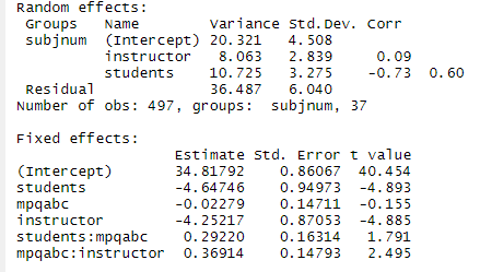
Model2

(d) Write the corresponding model out as Level 1 and Level 2 equations. (In terms of parameters, not estimates). How many parameters are estimated in this model?

 

  gives us the fixed effect for mpqabc

  gives us the instructor*mpqabc interction

gives us the students*mpqabc interction

We are also assuming we have .  Whether you use  or  notation isn’t that important but differentiating and remembering what they measure.

There are 6 “beta” coefficients, 4 variance terms, and 3 covariances. = 13 parameters.

 

(e) Provide interpretations for all estimated parameters!

·       34.82 is estimated pre-performance happiness for public or juried recitals for the average musicians with average MPQ absorption (or estimated population mean for population of musicians with average MPQ absorption)

·       -4.65 is the predicted decrease in pre-performance happiness for student audiences for a particular musician with average MPQ absorption (have to zero out the interaction) compared to public/juried audiences

·       -.02279 is the predicted decrease in pre-performance happiness associated with a one-unit increase in the MPQ absorption scale for public or juried recitals (have to zero out the interaction)

·       -4.25 is the predicted decrease in pre-performance happiness for an instructor  audience for a particular musician with average MPQ absorption compared to public/juried audience

·       .369 is the predicted lowering of the negative effect of instructor audience on pre-performance happiness as performer MPQ increases. (Note: slope of mpqabc = -.023 + .292 student + .369 instructor.  So if performing in front of an instructor, a one-unit increase in MPQ is associated with a -.023 + .369 = 0.35 increase in pre-performance happiness rather than a 0.023 decrease if performing in front of public/jury.)

·       .2922 is the lowering of the negative effect of student audience on pre-performance happiness as performer MPQ absorption increases (becomes less negative for student audience – in fact, if a student audience, a one-unit increase in MPQ absorption is associated with a 0.27 increase in pre-performance happiness)

·       20.32 is the musician to musician variability in pre-performance happiness for performers with average MPQ in a public or juried recital.

·       8.063 is the variability in the effect (slope) of an instructor audience (vs. public or juried) across musicians

·       10.725 is the variability in the effect (slope) of a student audience across musicians

·       36.587 is the unexplained variability across performances within musicians after adjusting for audience type and MPQ absorption

·       0.09 is a weak correlation between intercepts and the instructor slopes (estimated correlation between pre-performance happiness levels for juried recitals or public performances and changes in happiness for instructor audiences, after controlling for absorption levels)

No real fanning Cov = .09(4.508)(2.839) = 1.2 Min = 1.2/10.725 ≈ 0 (so fanning out if anything)   Knowing a musician’s intercept doesn’t tell us much about the impact on them of an instructor audience (might be larger or smaller than average)

 

·       -0.73 says musicians with higher intercepts (pre-performance happiness for public or juried recitals and average MPQ absorption) tend to have even larger decreases in happiness for student audiences than musicians with smaller intercepts.

Cov = -.73(4.508)(3.275) = -10.77 Min = 10.77/10.725 ≈ 1 (so fanning in)

 

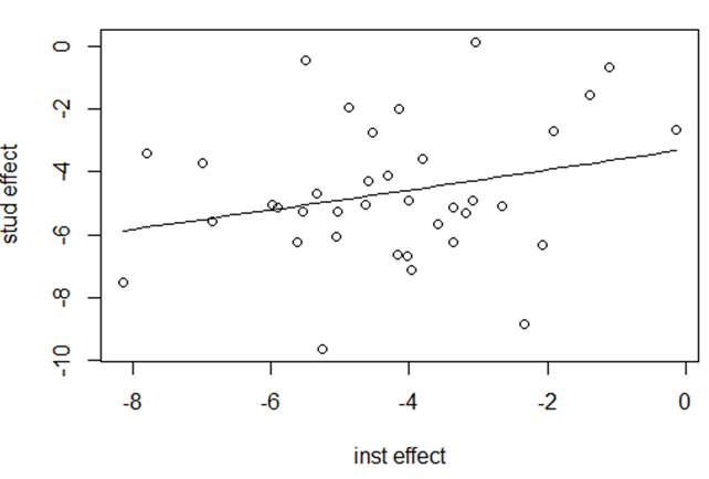
·       0.60 says musicians with a larger effect of instructor tend to have a smaller effect for student audiences. Let’s improve this answer:

Here is a graph of the student slopes vs. the instructor slopes.  Students that have lower na scores in front of instructors rather than public performances (large negative effect) tend to also have lower na scores in front of students rather than public performance (large negative effect).   Student in lower left: -8 when in front of instructor and -8 when in front of students.  Student in upper right: -1 when in front of instructor, -1 in front of students.

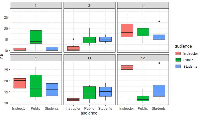
Subject 1 has large decreases for both or Subject 12 actually increases for both. Most others have small differences for both.  Few are like #3 and #11 where one type of audience is helpful but the other isn’t, or like 12 were they have a negative effect from instructor.

 

(f) Which variance components decreased the most between Model1 and Model2? Provide a brief interpretation.

The slopes for instructors and students.  So knowing MPQ absorption explains variation among musicians in the instructor-audience and student-audience effects.

 

(g) Suppose I want to add an indicator variable for male to Model 2 as a predictor for all intercept and slope terms. How many parameters will this add to the model?

 

This is a Level 2 variable.  So you will have 3 new level 2 coefficients (in each of the three Level 2 equations)

 

(h) Suppose I add the male indicator to Model 2 as suggested.  How will this change the interpretations you gave in (e)?

The intercept applies to females and the slope coefficient interpretations are after adjusting for both MPQ and gender.  When trying to zero out interaction terms will be talking about females with average MPQ absorption.

 

2) Kentucky Math Scores

Data were collected on 48,058 students from 235 middle schools from 132 different districts.  These students were Kentucky eighth graders who took the California Basic Educational Skills Test in 2007.  However, this analysis involves only 46,940 students who are complete cases.  The variables of interests from this data set are:

 - sch_id = School Identifier

 - nonwhite = 1 if student is Not White and 0 if White

 - mathn = California Test of Basic Skills Math Score

 - sch_ses = School-Level Socio-Economic Status (Centered)

 

Main Objective

Is there a difference in math scores of eighth graders in Kentucky based on ethnicity and socioeconomic status, after accounting for the multilevel nature of the data?

 

(a) Summarize what you learn from the following graphs

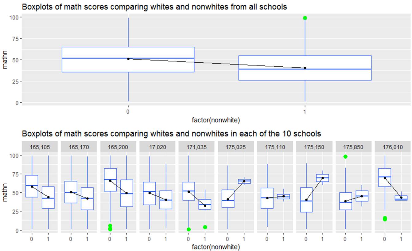
Overall, whites (nonwhite = 0) tend to have higher math scores than non whites (nonwhite = 1), but we see there is quite a bit of variation in this comparison across schools. In some schools (e.g., 175205 and 175150), the nonwhites actually score  quite a bit higher – though it also appears those are small sample sizes and may be a very selective group of test takers.  Maybe there is some characteristic of those school that might explain this change in slope.

 

(b) Summarize what you learn from the following graph (for the same 10 schools)

 

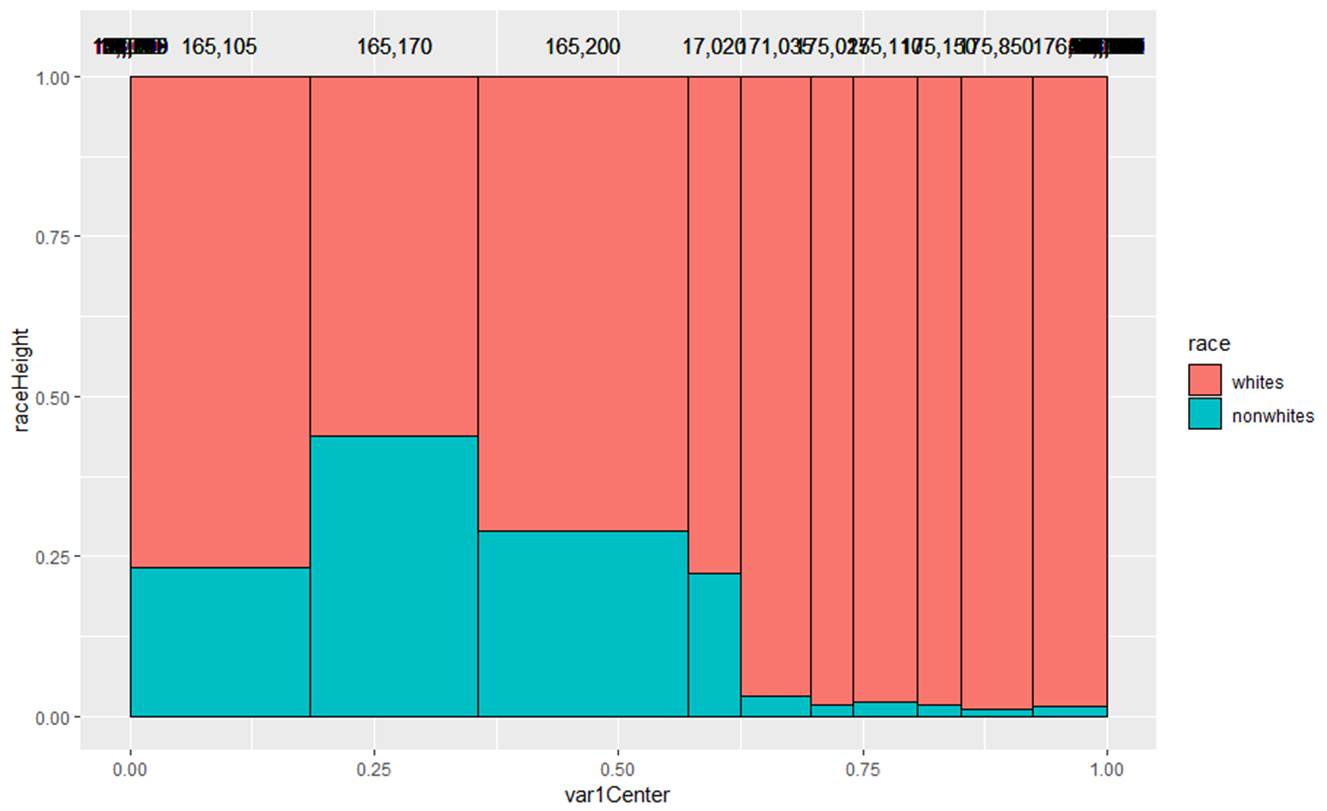This is graph is not very well labeled, it’s actually the racial breakdown for 10 of the schools.  The different width shows us the relative school size.  We see that the smallest schools have very few nonwhites, whereas the larger schools have the highest proportions of nonwhites in this sample.

 

(c) Summarize what you learn from the following graphs

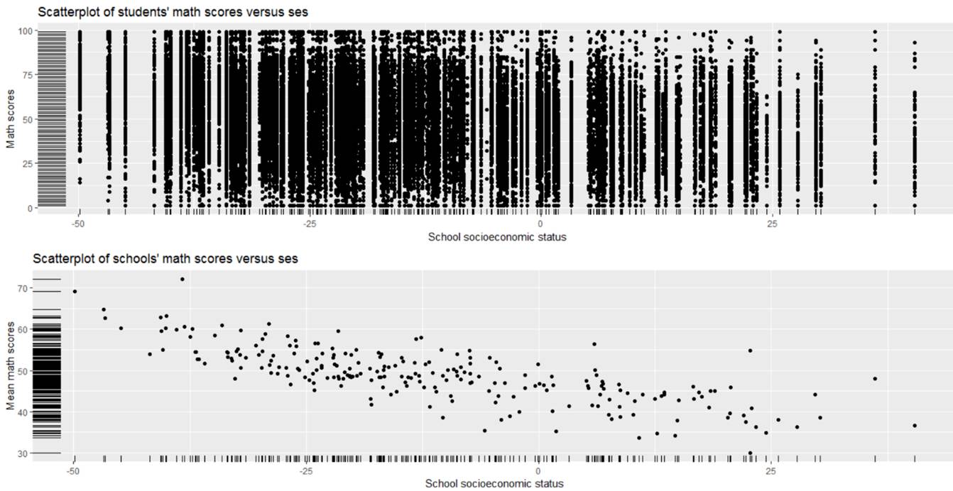
Overall there is a negative association between math score and the social economic status of the school though we see LOTS of within school variation in those math scores in the top graph.  The bottom graph (school-level averages) helps us see the overall trend but ignores that within school variability.

 

[It is kind of surprising to see that as ses increases, mean math scores tend to decrease.  A possible explanation is that this test is only for students at the basic level, hence the name “California Basic Educational Skills Test.”  So schools that are low ses have more basic level students taking it and they tend to do better.  However, schools that are high ses have fewer basic level students taking it and they tend to do worse?]

 

(d) For each school separately, I have run a traditional regression to predict math score from student race (1 = nonwhite, 0 = white).  For each school, I saved the intercept and slope of that regression.  Below are the results

> summary(intercepts)    Min. 1st Qu.  Median    Mean 3rd Qu.    Max.    31.0    45.9    49.8    50.1    54.3    77.4 > summary(slopes)    Min. 1st Qu.  Median    Mean 3rd Qu.    Max.    NA's -34.190 -14.986  -8.610  -6.799   0.061  34.955      21

 

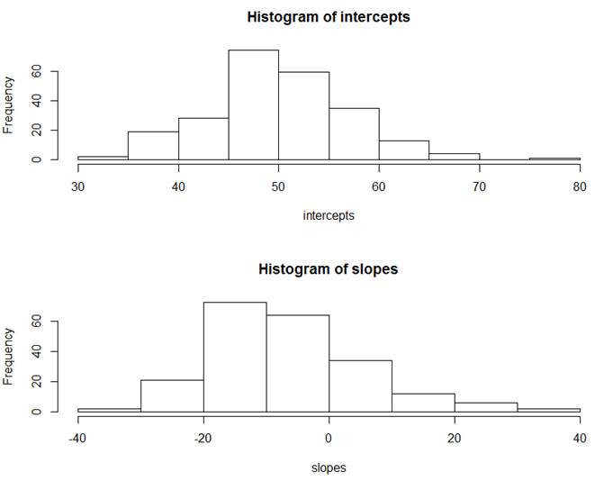
Briefly summarize what you learn.

The intercepts represent the predicted math scores for white students (nonwhite = 0).  We see that the predicted math scores for white students is about 50.1 pts on average across all schools.  The slopes represent the difference in the predicted math scores from the whites to the nonwhites. We see that nonwhites are estimated to have a lower math score than whites by 6.8 pts on average across all schools. But we see lots and lots of variability in these slopes and intercepts across the schools. The SD for intercepts is about 7 pts and the SD for the slopes is about 12 pts.  About 25% of the schools have a positive slope (higher average scores for the nonwhites).

Below are the group means and standard deviations from the raw data, without adjusting for the schools.  Notice this would have estimated about 12-13 points lower for the nonwhites on average.

> summary(math$mathn[math$nonwhite == 1])

   Min. 1st Qu.  Median    Mean 3rd Qu.    Max.

    1.0    26.0    39.0    40.8    55.0    99.0

> summary(math$mathn[math$nonwhite == 0])

   Min. 1st Qu.  Median    Mean 3rd Qu.    Max.

    1.0    36.0    52.0    51.1    65.0    99.0

 

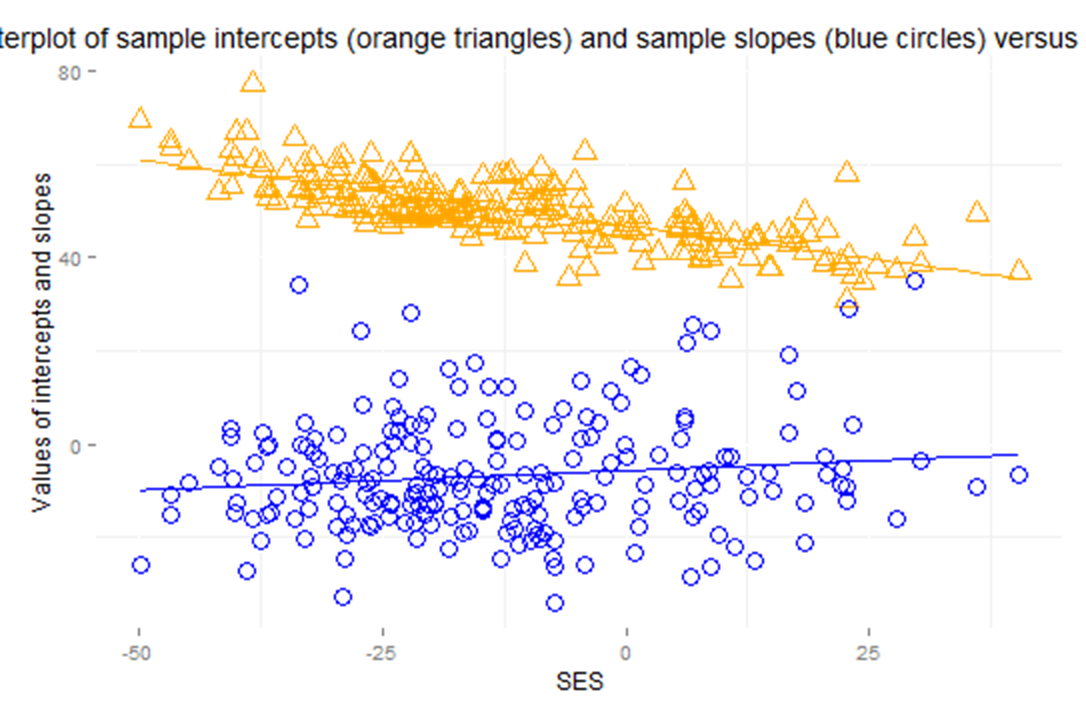
(e) Summarize, in context, what you learn about the association between the slopes and intercepts.

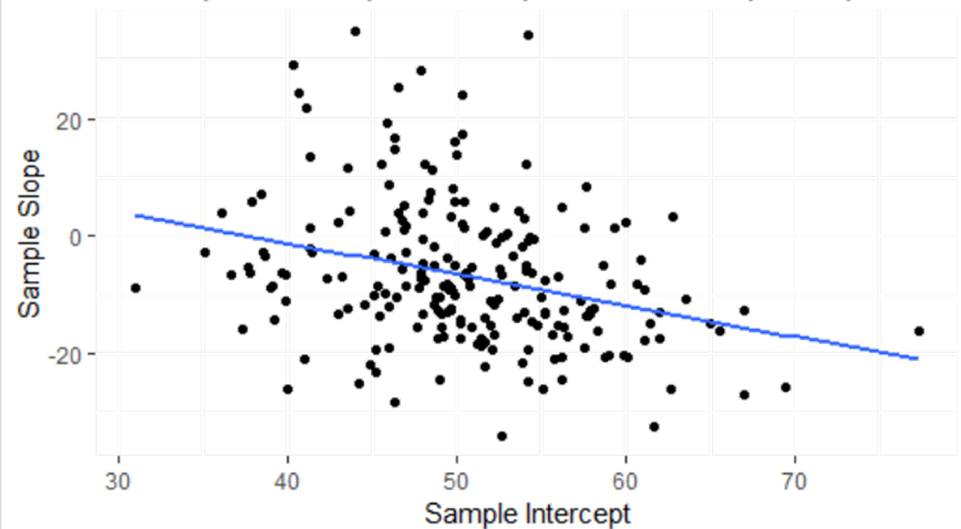
As sample intercepts increase, sample slopes tend to decrease.  In context, for schools where the predicted math score for white students is above average, the difference between the whites and nonwhites becomes increasingly negative (larger difference between the whites and nonwhites).  In schools where the predicted math score for white students is below average, the slopes are closer to zero, meaning there is less of a race gap.

(f) Describe the nature of the association between ses and the sample intercepts and between ses and the sample slopes.  Is there preliminary evidence that ses is a good predictor of the sample intercepts and sample slopes based on the associations? [Hint: What do these slopes represent?]

As school ses increases, the predicted math scores for white students (intercepts) decrease and the difference between whites and nonwhites gets less negative (closer to zero). Interpretation: Nonwhites tend to benefit from higher ses more than whites in regards to higher predicted math scores.  Yes, there is preliminary evidence that SES will be helpful to the model, stronger for intercepts than slopes. 

(g) Below is output from regressing the intercepts on the school SES and then from regressing the slopes on the school SES.

 Summarize what you learn.

> model.intercept = lm(intercepts ~ mean.ses$x)

> summary(model.intercept)

Call:

lm(formula = intercepts ~ mean.ses$x)

Residuals:

    Min      1Q  Median      3Q     Max 

-13.112  -3.349  -0.659   2.549  19.742 

Coefficients:

            Estimate Std. Error t value Pr(>|t|)    

(Intercept)  46.8675     0.3616   129.6   <2e-16 ***

mean.ses$x   -0.2811     0.0166   -16.9   <2e-16 ***

---

Signif. codes:  0 ‘***’ 0.001 ‘**’ 0.01 ‘*’ 0.05 ‘.’ 0.1 ‘ ’ 1

Residual standard error: 4.71 on 233 degrees of freedom

Multiple R-squared:  0.551,   Adjusted R-squared:  0.549 

F-statistic:  286 on 1 and 233 DF,  p-value: <2e-16

> model.slope = lm(slopes ~ mean.ses$x)

> summary(model.slope)

 

Call:

lm(formula = slopes ~ mean.ses$x)

 

Residuals:

   Min     1Q Median     3Q    Max

-27.86  -7.48  -1.97   7.55  42.78

 

Coefficients:

            Estimate Std. Error t value    Pr(>|t|)   

(Intercept)  -5.7084     1.0210   -5.59 0.000000069 ***

mean.ses$x    0.0847     0.0460    1.84       0.067 . 

---

Signif. codes:  0 ‘***’ 0.001 ‘**’ 0.01 ‘*’ 0.05 ‘.’ 0.1 ‘ ’ 1

 

Residual standard error: 12.2 on 212 degrees of freedom

  (21 observations deleted due to missingness)

Multiple R-squared:  0.0157,  Adjusted R-squared:  0.0111

F-statistic: 3.39 on 1 and 212 DF,  p-value: 0.0671

 

Every one unit increase in school-level ses is associated with a .281 decrease in the predicted math scores for whites, on average.

 

Every one unit increase in school-level ses is associated with a decrease in the whites’ “advantage” over nonwhites by .08467 (what was a negative coefficient becomes less and less negative).

Is either association statistically significant? How much of the variation in intercepts and slopes is explained by the school SES?

The school SES is a highly significant predictor of average math scores for whites (explaining 55% of the variation in intercepts) and is borderline significant for the change in average math scores between nonwhites and whites (explaining 1.6% of the variation in slopes).

(h) How do the above results compare to the “unconditional means” (null, random intercepts only) model?

> lmer(mathn ~ 1 + (1 | sch_id), REML=TRUE, data=math)

Linear mixed model fit by REML ['lmerMod']

Formula: mathn ~ 1 + (1 | sch_id)

   Data: math

REML criterion at convergence: 416975

Random effects:

 Groups   Name        Std.Dev.

 sch_id   (Intercept)  6.32   

 Residual             20.40   

Number of obs: 46940, groups:  sch_id, 235

Fixed Effects:

(Intercept)  

         49  

The predicted overall mean math score for the average school is 49 (similar to the 46.87).  The estimated within school variation in students’ math scores (from the mean) is 20.40.  = 6.32, this is the school to school variability in the mean math scores (compare this to the standard deviation of the intercepts found above)

 > sd(intercepts)

[1] 7.0059

 

(i) Calculate and interpret the intraclass correlation coefficient.

6.32²/(6.32² + 20.40²) = .0875

 

So this is not that large, which says there isn’t that much school-to-school variability relative to the variability in the scores within the same school, that there is much more variability among the students within a school than there is among schools. Remember how much “cleaner” the graph of the means was compared to the graph of math score for individual students.

 

So if we go back to the first set of boxplots, we see that math scores ranges from 0 to 100, but the school means were all pretty much in the 40-60 range. Taking the school ID into account doesn’t explain much of the variability in the data.

 

(j) Below is the multilevel model version of the analysis.

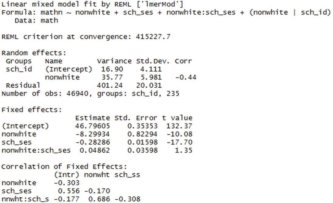
Interpret each estimated parameter.

 = 46.8, this is our overall estimate the mean math score for whites for the average school with average SES.

 

 = -8.3 this is the predicted change (decrease) in mean math scores for nonwhites compared to whites in a particular school with sch_ses = 0 (at the mean SES)

 

 = -0.283 this tells us the predicted change (decrease) in mean math scores with a one-unit increase in school SES for whites (nonwhite = 0)

 

 = 0.0486 = this tells us about the difference in the effect of SES for whites and nonwhites.  For whites, the overall effect of SES is negative (-.283). For nonwhites, the overall effect of SES is less negative (-2.83 + .0486).  Similarly, as the SES increases, the difference between whites and nonwhites decreases (-.8299 + .0486 SES).

 

 16.90 = this tells us about the school-to-school variation in mean math scores for whites after adjusting for SES (compare the square root to the SD of the intercepts)

 

 35.77 this tells us about the school-to-school variation in the race effect (difference in mean math scores for whites and nonwhites), after adjusting for SES (compare square root to SD of the slopes)

 

 -0.44 = the correlation between the slopes and intercepts. The negative value shows that as the intercepts decrease (lower avg scores for whites) the slope coefficient increases (becomes less negative in this case as there is less of a distinction between whites and nonwhites).

 

Notice how much the variance in the intercepts has decreased by bringing in the school SES, now on par with the variation in the slopes.

 

(k) Which predictors would you consider significant? Are the results consistent with what you learned in (g)? Explain.

The main effects of ses and race are significant but the interaction between the two is not (though more evidence here than in if we don’t account for the clustering in the data, see next question).

 

There is evidence that math scores differ by race and by ses separately, but the difference in math scores between whites and nonwhites is not modified by ses (the regression of the slopes on SES was not a strong association, but the regression on the intercepts was).

 

(l) Below is a “one-level” analysis of the data, ignoring the school IDs. 

> summary(lm(math$mathn ~ math$nonwhite + math$sch_ses + math$nonwhite:math$sch_ses))

Call:

lm(formula = math$mathn ~ math$nonwhite + math$sch_ses + math$nonwhite:math$sch_ses)

Residuals:

   Min     1Q Median     3Q    Max 

-58.12 -14.48   0.39  14.14  65.96 

Coefficients:

                            Estimate Std. Error t value Pr(>|t|)    

(Intercept)                 46.39809    0.13353  347.48   <2e-16 ***

math$nonwhite              -10.36714    0.40456  -25.63   <2e-16 ***

math$sch_ses                -0.30420    0.00562  -54.13   <2e-16 ***

math$nonwhite:math$sch_ses   0.00984    0.01771    0.56     0.58    

---

Signif. codes:  0 ‘***’ 0.001 ‘**’ 0.01 ‘*’ 0.05 ‘.’ 0.1 ‘ ’ 1

Residual standard error: 20.5 on 46936 degrees of freedom

Multiple R-squared:  0.0881,  Adjusted R-squared:  0.088 

F-statistic: 1.51e+03 on 3 and 46936 DF,  p-value: <2e-16

Do any of the conclusions change?

Now we would see very little evidence of an interaction, though other conclusions are similar.

(m) Why do you think our conclusion about the significance of the SES x race interaction is so different between these two approaches?

In the separate regressions exploration, we saw a bit more evidence of an interaction (significance of SES in the slopes, p-value = .067) and we see no evidence of an interaction in the one-level model (p-value = 0.58).  The one-level model has not accounted for any school-to-school variation and this makes it more difficult to detect the subtle interaction.  The separate regressions doesn’t do any “pooling together” of information across the schools. The multilevel model is “between.”  A small school with a large difference between whites and non-whites may be down-weighted a bit based on what is going on at the other schools.

 

3) Consider the NLSY data on children’s anti social behavior (measured in 1990, 1992, 1994).

(a) Suppose we fit an ordinary least squares (OLS) regression to the data, Y_ij= X +  with

Note: The residual standard error for this model is  = 1.51.

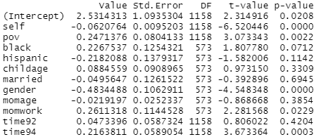
What do we consider to be the main flaw in this analysis?  What do we expect to be the main consequence of this flaw?

This ignores the clustering of the data from repeat observations on each individual. We expect this to “deflate” our estimate of the standard errors of the coefficients and make relationships look more significant than perhaps they should (like we had a larger sample size).  

The coefficient of poverty tells us about the “marginal association,” averaging the poverty effect across all the individuals without taking into account individual to individual differences.

(b) Suppose we fit the following model: Y_ij = X +  with . So i  refers to the 3 time points and we are allowing the variability of the measurements in 90 to differ from 92 and 94 and we are allowing each of the three pairs of measurements to have different correlations.  Note: using the data in wide format, we find corr(90,92) = 0.64, corr(90, 94) = .54, corr(92, 94) = 0.60.  We also find var(time90) = 2.16 (sd = 1.47), var(time92) = 2.43 (sd = 1.56), and var(time94) = 2.86 (sd = 1.69).  The gls command allows us to fit this very flexible model.

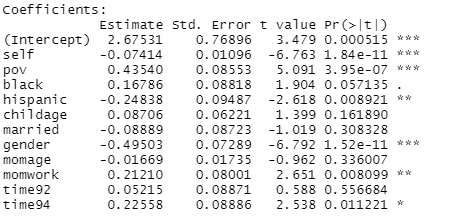
model1a = gls(anti ~ self + pov + black + hispanic + childage + married + gender + momage + momwork + time,

             corr = corSymm(form = ~ 1 | id), weights = varIdent(form = ~1 | time), method="ML", data = nlsy_long)

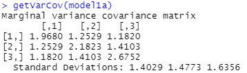
So we are assuming different correlations between pairs of measurements (corr by id) at different times (there are three rho-hats in the output) and variances that change across the three time points (var by time) (there are 3 parameter estimates,  = 1.403,  = 1.403 x 1.053…).

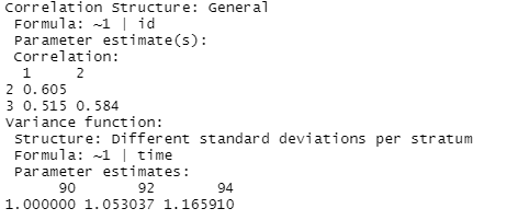
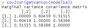
Explain what the parameter estimates of 0.605, 0.515, and 0.584 represent. Explain what the parameter estimates of 1.00, 1.05, and 1.165 represent.  How many total parameters are estimated in this model? 

The parameter estimates are the correlations of the residuals and the multipliers (e.g.,  = 1.403). This allowed for “unstructured” variances and “unstructured” covariances. There are 18 parameters, the 1 intercepts, 11 fixed effects, 3 correlations, and 3 variances).

0.605 is the esitmated correlation between the time90 and the time92 observations. 

0.515 is the estimated correlation betweenthe time90 and the time94 observations.

0.584 is the estimated correlation between the time92 and the time94 observations.

1.402865 is the estimated standard deviation of the time90 observations.

1.053 x 1.4029 = 1.48 is the estimated standard deviation of the time92 observations.

1.1659 x 1.4029 = 1.64 is the estimated standard deviation of the time94 observations.

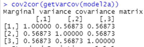
Bonus question: what will the variance-covariance matrix for this model look like?  How will it compare to the same matrix in (a)? How many parameters are estimated?

The variance-covariance matrix in (a) will have the estimated value of  along the diagonal and zeros everywhere else.

The variance-covariance matrix in (b) will have 1.403², 1.48², and 1.64² along the diagonal, and the off diagonals will represent the covariances, e.g., .605*1.403*1.48 = 1.26; .515*1.403*1.64 = 1.18.

The gls command only allows us to see the “marginal” variance-covariance and correlation matrices, so about the “y’s.”  (There is no separation of the within person and between person variability.)

(c) Suppose we fit the following model: : Y_ij = X +  with .  

model2a = gls(anti ~ self + pov + black + hispanic + childage + married + gender + momage + momwork + time,    corr = corCompSymm(form = ~ 1 | id),   weights = varIdent(form = ~1 | time), method="ML", data = nlsy_long)

 

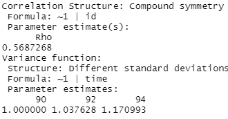
Explain the model implications.

 

“Compound symmetry” means we assume the same correlation for all pairs of observations, estimated as 0.568, rather than allowing for different correlations among different pairs.  This is what is meant by exchangeability. So it doesn’t matter how far apart the years are, or what the two years are in the pair, the same correlation coefficient. This would match the ICC.  We are still allowing for unequal variances and the multipliers have changed a bit, but still increasing variability in later years.

 

Bonus question: what will the variance-covariance matrix for this model look like?  How will it compare to the others?  How many parameters are estimated?

This model has one parameter for the correlation rather than 3.

 So now we have

1.408 as the estimated standard deviationof time90 observations,

1.408*1.0376 = 1.46 for time92 and 1.408*1.17099 = 1.65 for time94

And the off diagonals be 0.569*1.408*1.46 = 1.17,  0.569*1.408*1.65 = 1.32, and 0.569*1.46*1.65 = 1.37.

 

 

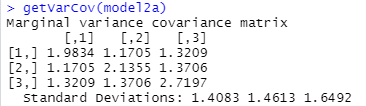
If the variances had been the same, then the off diagonal entries in the covariance matrix would have all matched as well.

 

(d) Suppose we fit the following model: Y_ij = X +  with  

model3 = lme(anti ~ self + pov + black + hispanic + childage + married + gender + momage + momwork + year, random = ~1 | id,  method= "ML", data = nlsy_long)

 

Now Var(Y_ij) =  and  (the epsilons are not correlated, and the epsilons and u’s are not correlated)

 

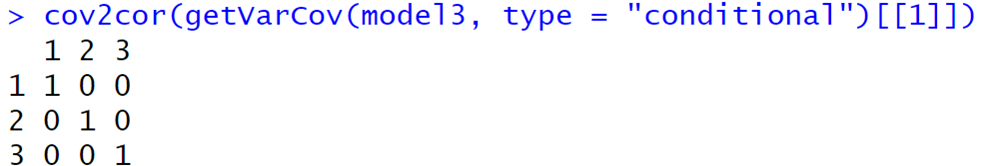
What is the intraclass correlation coefficient?  What does the variance-covariance matrix for this model look like?

 1.133²/(1.133² + .9964²) = 0.564 (after adjusting for the variables in the model, this is how correlated two observations would be, note the similarity to model2a). But this model has random intercepts and not random slopes, so we also are assuming the variability is the same in each year, so the diagonals will all be .9964² + 1.1325²= 2.28 and the off-diagonals will all be the same (.564*2.28 = 1.28)

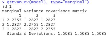
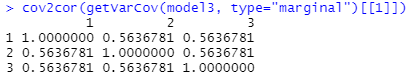
So the correlation of any pair of observations on the same individual is estimated to be 0.564 (rather than zero).

 

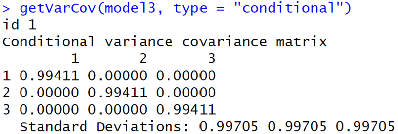
Now we can ask R for the “conditional” matrices as well, = 0.993 » 0.9964² and we have “conditional independence” of the errors within each individual.

 

 

(e) The model in (c) matches what we get from the random intercepts model for the correlation matrix for the model in (d), but the random intercept model assumes equal variances. How would I adjust the multilevel model to allow for unequal variances?

Random slopes

 

(f) The resulting standard errors from the multilevel model (from d) are considered more valid.

How do these standard errors compare to the ols model?

Generally larger

Also notice that the coefficient of poverty has changed … here is represents the effect for the “average person,” conditional on all the other variables.

 

The “fixed” model below includes the children id in the model as a fixed effect.  This adjusts the standard errors for dependence and controls for all stable characteristics of the individuals.

(g) The fixed effects model does not include any Level 2 variables.  Why not? (Though we could include interactions with level 2 variables.)

Because we could have complete confounding between the “id variable” and any variable about the children.

 

(h) This noticeably changes the poverty coefficient.  How would you now interpret the coefficient? How has the standard error for poverty changed?

For a particular child in our dataset, changing from not in poverty to in poverty predicts an increase of 0.112 in anti-social behavior.  The standard error is a bit larger (.093 vs. .0804)   

In fact, we would not consider this poverty variable to be statistically significant (.112/.093 < 2).

In the random effects model, we interpret the poverty coefficient as the difference in the predicted mean anti-social behavior between two populations of children, one group in poverty, one group not in poverty, where all the other characteristics (e.g., black, momwork) are the same between the two populations. This difference is significant (t > 2).

 

More quotes!

·       Fixed effects methods only use variation within individuals to estimate coefficients.

·       Like estimating separate regressions for each person, then averaging the regression coefficients across persons (NB: can’t actually do this here because number of predictors is greater than the number of time points)

·       A consequence is that standard errors tend to be larger for FE models

·       Each individual serves as his or her own control

In sum, FE methods reduce “omitted variable” bias but at the expense of increased standard errors. If there’s very little variation within individuals, FE methods will not produce reliable estimates.

 

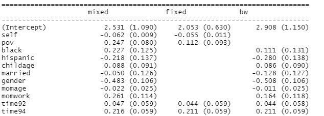
We discussed the “Hausman test” before as a comparison of these two models to see whether the mixed effects model (random effects) adequately accounts for all important potential Level 2 variables (no confounding between a Level 1 variable and something at the group level.)  A hybrid approach is called a “between-within” model (bw). The bw model is again just our mixed model with both level 1 (deviation) and level 2 variables (group mean).

(i) How does the coefficient of poverty compare between the 3 models? (Hint: Which is it equal to and why?)

The “within child” coefficient doesn’t change (because we have already accounted for the child-to-child differences in the fixed effects model, but the “between child” coefficient now captures the between group association.

(j) Does there appear to be a practical and/or significant difference between the “within” effect of poverty and the “between” effect of poverty? How are you deciding? Which is worse, changing poverty status or being a person in poverty?

The between child slope is 0.616, much larger than the within-child slope (0.112).  So a child changing poverty status doesn’t seem to have much of a significant effect, but being a child in poverty vs. not in poverty does have a significant effect, on average (Its effect is larger between children than within children.)

 

Let’s just compare the models with self, pov, and year, and whether or not we include the id variable and whether or not we include the “group-mean centered” poverty variable and the deviation variable.

	lm(anti ~ self + pov + year)	lm(anti ~ self + pov + year + factor(id))	lmer(anti ~ self + pov + year + (1 | id))	lmer(anti ~ self + pov_d + year + (1 | id)	lmer(anti ~ self + pov_d + pov_gmj + year + (1 | id)	lmer(anti ~ self + pov + pov_gmj + year + (1 | id)
	No id	Id as fixed	Id as random	With	With  and	With  and
Slope of pov	0.518	0.113	0.295	0.113	0.113, 0.692	0.113, 0.579
Interpretation	Average across everyone, ignores group differences	“averaged” within subject effect (“subjects act as their own controls”, have “discarded” all between group variance) More appropriate if only interested in Level 1 variables? (e.g., small # of clusters)	Within and between subject (can explain variation at both levels, with same ). Assumes  Adjusts the group mean for the Level 1 variable.	Within subject (assumes no between group variance) Typically gives larger  (not adjusted).	Separates within subject and between subject (e.g., being an educated person vs. living in an educated country) “Between-within model”	.692 - .113 = .579 (the addition if group mean increases but pov held fixed) (if zero, go back to column 3, Hausman test)

 

 

 

4)

(a) Write out the Level 1 and Level 2 equations, including variance/covariance components. 

With random intercepts and random slopes:

Level 1: foul.diff_ij

Level 2:  and

with  and

 

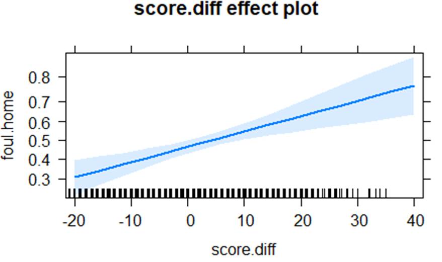
(b) Interpret the sign of the foul.diff slope. Does it support the conjecture?

The coefficient of foul.diff is negative indicating that in a particular game, the probability of a foul being called on the home team decreases as the foul-differential increases (more fouls being called on home time).

 

The slope is pertinent to a specific game, turns out to be much larger than when if treat the calls in the same game as independent (a single level model ignoring the game). Also note that the standard errors are likely larger in the multilevel model, this often happens when we account for correlated observations, essentially reducing the sample size.

 

(c) Now consider the following model with crossed random effects

> summary(model3 <- glmer(foul.home ~ foul.diff + (1 | game) + (1 | hometeam) + (1 | visitor), family = binomial, data = bball) )

Generalized linear mixed model fit by maximum likelihood (Laplace

  Approximation) [glmerMod]

 Family: binomial  ( logit )

Formula:

foul.home ~ foul.diff + (1 | game) + (1 | hometeam) + (1 | visitor)

   Data: bball

 

     AIC      BIC   logLik deviance df.resid

  6780.5   6813.0  -3385.2   6770.5     4967

 

Scaled residuals:

    Min      1Q  Median      3Q     Max

-1.6589 -0.9056 -0.6522  0.9679  1.7952

 

Random effects:

 Groups   Name        Variance Std.Dev.

 game     (Intercept) 0.17165  0.4143 

 hometeam (Intercept) 0.06809  0.2609 

 visitor  (Intercept) 0.02323  0.1524 

Number of obs: 4972, groups:  game, 340; hometeam, 39; visitor, 39

 

Fixed effects:

            Estimate Std. Error z value Pr(>|z|)   

(Intercept) -0.18780    0.06331  -2.967  0.00301 **

foul.diff   -0.26385    0.03883  -6.795 1.08e-11 ***

 

BTW, interpreting the coefficients:

The log odds of a foul being called on the home team, when the foul differential is zero, for the average game, average hometeam, and average visitor, are estimated to be -0.1878.

           Estimated odds: exp(-0.1878) = 0.829

           Estimated probability: 0.829/(1+0.829) » 0.45 (slightly more likely for a foul to be called on the visiting team)

 

As the foul differential increases, the estimated log-odds decrease by -.26385, for a particular game, home team, and visiting team.

odds decrease by a factor of exp(-.26385) = 0.768 (23% decrease)

 

We have significant evidence that the odds that a foul is called on the home team shrinks as the home team has more total fouls compared to the visiting team at a particular point in the game.

 

How much of the variation is due to differences game to game? How much due to differences among the home teams, and how much due to differences among the visiting teams?

Game: .17165/(.17165 + .06809 + .02323) = .653

Home: .06809/(.17165 + .06809 + .02323) = .259

Visitor: .02323/(.17165 + .06809 + .02323) = .088

 

Note, you could include 3.29 in each denominator if you wanted that to reflect “within game/home/visitor” variation…

 

(d) Explain, in context, what it means for a team to have a large positive random effect (largest are Depaul and Seton Hall) or a large negative random effect (e.g., Purdue, Syracuse).

When they are the home team, Depaul and Seton Hall tend to see more fouls called on them, Purdue and Syracuse the least.

 

 

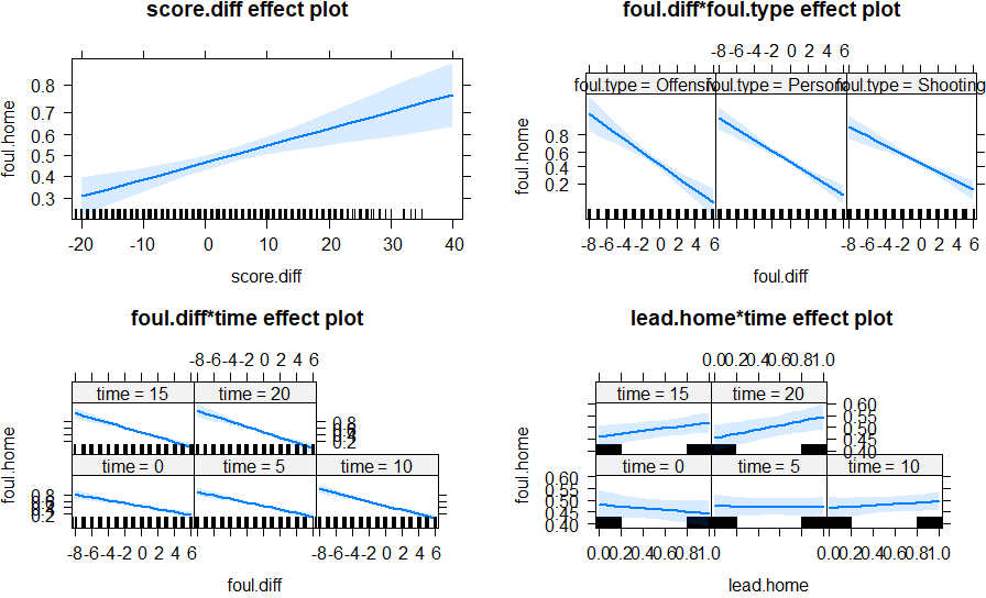
Now consider a model that accounts for score differential, whether the home team has the lead, time left in the first half, type of foul, the interaction between foul differential and type of foul, the interaction between foul differential and time, and the interaction between home team lead and time, with random intercepts for game, home team, and visiting team.

summary(model5 <- glmer(foul.home ~ foul.diff + score.diff + lead.home +

      time + foul.type + foul.diff:foul.type +  foul.diff:time + lead.home:time + (1 | game) + (1 | hometeam) + (1 | visitor),  family = binomial,     data = bball))

              exp(fixef(model5))

Fixed effects:

                             Estimate Std. Error z value Pr(>|z|)   

(Intercept)                 -0.328087   0.157636  -2.081  0.03741 * 

foul.diff                   -0.274966   0.062215  -4.420 9.89e-06 ***

score.diff                   0.033515   0.008236   4.069 4.72e-05 ***

lead.home                   -0.150126   0.177231  -0.847  0.39696   

time                        -0.008693   0.008561  -1.015  0.30992   

foul.typePersonal            0.148216   0.108605   1.365  0.17234   

foul.typeShooting            0.081163   0.111237   0.730  0.46561   

foul.diff:foul.typePersonal  0.047689   0.052306   0.912  0.36191   

foul.diff:foul.typeShooting  0.103333   0.053867   1.918  0.05507 . 

foul.diff:time              -0.008700   0.003274  -2.657  0.00788 **

lead.home:time               0.025947   0.012173   2.132  0.03304 * 

 

BTW, interpreting the fixed effects

The likelihood of a foul being called on the home team…

•        …increases when the home team is further ahead (and this effect doesn’t seem to depend on the foul differential as the interaction was not included here because it was not significant), after controlling for foul differential, type of foul, whether or not the home team has the lead, and time remaining in the half.  So referees are more likely to call fouls on the home team when the home team is leading and vice versa.

The rest are involved in interactions, so the coefficient shown is for a particular case.

•        … decreases as more fouls are called on the home team (when foul diff is a large negative; the odds of a foul on the home team increase, when foul diff is a large positive- more fouls on the home team compared to visitor- the odds of a foul on the home team decreases) - for offensive fouls, at halftime, after controlling for the effects of score differential and whether home team has the lead, but interactions don’t seem very significant, see graphs below)

•        … decreases if the home team has the lead, at half time (not significant)

•        … decreases as the number of minutes left in the first half increases (earlier in game), when the visiting team is leading and the foul differential is zero. In other words, if the game is closer to half time and the visiting team is ahead, then the likelihood of a foul being called on the home team increases. (not significant)

•        … larger for personal and shooting fouls compared to offensive fouls when foul differential is zero. (not significant)

 

Only foul differential and score differential are significant. (We should really run an ANOVA to be sure for foul type, see below, but personal and shooting have similar coefficients.)

 

 

(e) Summarize the signs of the coefficients of the interactions.

•    The negative “effect” of the foul differential on the likelihood of the next foul being called on the home team is smaller (less negative) for personal fouls and even less negative for shooting fouls (could be significant? Check anova table) and larger/more negative (missing coefficient is negative) for offensive fouls. (This supports the hypothesis that the evening out behavior is more noticeable for the calls over which the referees have more control, especially offensive calls which are much more of a judgement call.) … after controlling for score differential, whether the home team has the lead, and time remaining.

•    The negative effect of the foul differential on the likelihood of the next foul being called on the home team is smaller (less negative) when the game is closer to half time, after controlling for foul differential, score differential, whether the home team has the lead, and type of foul. (So a large differential early in the first half increases the odds of a foul on the home team even more; they seem to try and even things out more earlier in the game.)

•    When the game is close to half time, the home team is less likely to have a foul called on them when they have a lead then when they don’t have the lead. However, earlier in the game, the probability of a home team fall is larger when the home team has the lead then whey they don’t.

 

 

 

5) Teen alcohol use

Curran, Stice, and Chassin (Journal of Consulting and Clinical Psychology, 1997) collected data on 82 adolescents at three time points starting at age 14 to assess factors that affect teen drinking behavior. Key columns in the data set are:

·       id = numerical identifier for subject

·       age = 14, 15, or 16

·       coa = 1 if the teen is a child of an alcoholic parent; 0 otherwise

·       male = 1 if male; 0 if female

·       peer = a measure of peer alcohol use, taken when each subject was 14. This is the square root of the sum of two 6-point items about the proportion of friends who drink occasionally or regularly.

·       alcuse = the primary response. Four items—(a) drank beer or wine, (b) drank hard liquor, (c) 5 or more drinks in a row, and (d) got drunk—were each scored on an 8-point scale, from 0=“not at all” to 7=“every day.” Then alcuse is the square root of the sum of these four items.

Primary research questions included:

·       Do trajectories of alcohol use differ by parental alcoholism?

·       Do trajectories of alcohol use differ by peer alcohol use?

 

(a)  Identify Level One and Level Two predictors.

Level 1: age (time)

Level 2: coa, male, peer

 

(b)  Run an unconditional growth model with age as the time variable at Level One. (include time and random slopes for time)  Interpret the intercept.

model1 = lmer(alcuse ~ 1 + age + (1 + age | id), data = alcohol)

 

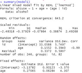
The intercept, -3.14, represents the predicted alcohol use for the average teen at age = 0.  Estimating the alcohol use for age = 0 (newborn) doesn’t make a lot of sense in this context!

It’s also for “square root of the sum of four items,” which doesn’t make much sense either!

 

(c)   Create age14 = age-14. Explain the advantage of doing so.

age14 = alcohol$age-14

Now the intercept will represent the predicted alcohol use at age = 14.

 

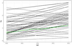
(d)  Rerun the unconditional growth model using age14, how do things change? (model1) Calculate and interpret an R² value for the Level 1 variance comparing this model to the null model.

model1 = lmer(alcuse ~ 1 + age14 + (1 + age14 | id), data = alcohol)

 

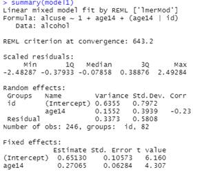
The intercept changes (now the predicted alcohol use – on average – for age 14).  This also changes the variance in the intercepts.  The original negative correlation implied lines were fanning in, indicating less variation in alcohol use at age 14 than age 0.

(The quadratic variance function would be minimized at age14 = .23(.7972)*(.3939)/.1552) = 0.465 or age = 14.465.  So these lines are starting to fan out again, so we predict the variability to be increasing for ages 15 and 16.)

 

The residual variance in the null model was .5617, which is now .3373 after adding age to the model (changing intercept definition doesn’t impact this), so the linear time trend explained (.5617 - .3373)/.5617 or about 40% of the within-person variation in alcohol use.

 

(e)  Add the effects of having an alcoholic parent and peer alcohol use in both Level Two equations to model1.

Adding these to both Level 2 equations means include them and their interactions with age14.

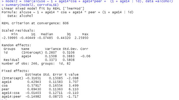
Report and interpret all estimated fixed effects, using proper notation (Think about what the graphs will look like)

 

Fixed effects:

·       Intercept : At age = 14, with no alcoholic parents, and no peer usage, we predict -.316 for alcohol use for the average subject.

·       Age14 : For the average teen with no alcoholic parents and no peer usage, we predict the alcohol use to increase, on average, by 0.429 each year.

·       Coa : At age 14 and after adjusting for peer usage, teens with alcoholic parents are predicted to have alcohol use 0.579 larger, on average, than teens without alcoholic parents, on average.

·       Peer : At age 14 and after adjusting for whether or not have alcoholic parents, teens with more peer usage tend to have more alcohol use themselves, on average.

·       Age14:coa : After controlling for peer alcohol use, the year by year increase in alcohol use is predicted to be smaller (.014 pts) for teens with alcoholic parents than without alcoholic parents on average (but not significant).

·       Age14:peer : After controlling for parental alcoholism, the year by year increase in alcohol use is predicted to be smaller as the level of peer usage increases, on average.

 

These Level 2 variables appear to explain more variation in the intercepts than in the slopes and we might consider simplifying this model by removing the interactions between age and coa and between age and peer (though interaction with peer is a bit more significant, because we did see higher peer usages corresponding a bit to smaller slopes, hence negative coefficient). 

 

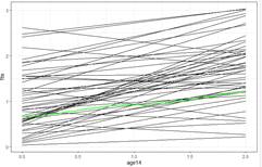
“Raw data” (with smoothers) for peer usage

 

(peer = 1 has higher intercept but flatter slope though not statistically significant in above model)

 

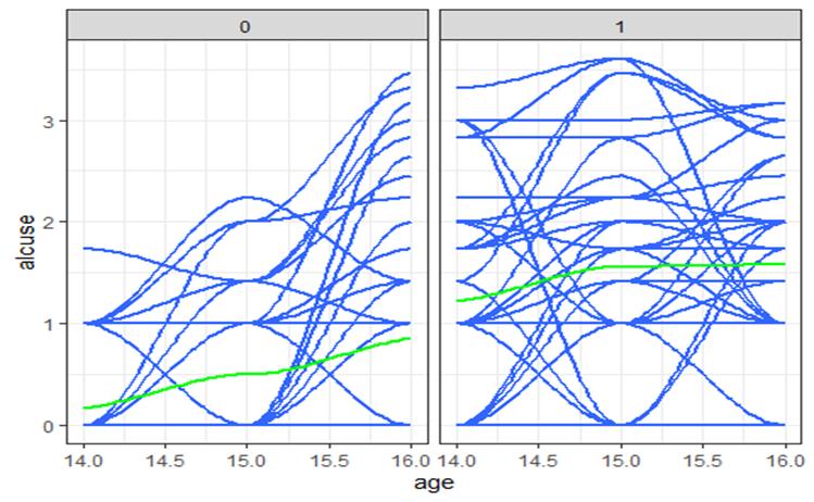
“Raw data” (with smoothers) for COA

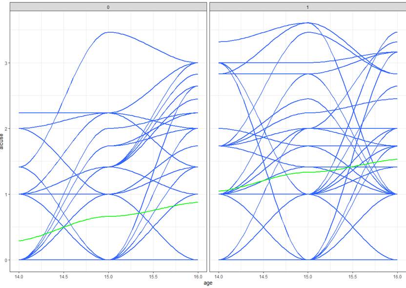
(if parents alcoholic, higher intercept and flatter slope)

 

 

6) Chapp et al. (2018) explored 2014 congressional candidates’ ambiguity on political issues in their paper, Going Vague: Ambiguity and Avoidance in Online Political Messaging. They hand coded a random sample of 2012 congressional candidates’ websites, assigning an ambiguity score. These 2014 websites were then automatically scored using Wordscores, a program designed for political textual analysis. In their paper, they fit a multilevel model of candidates’ ambiguities with predictors at both the candidate and district levels.

Variables of interest include:

·       ambiguity = assigned ambiguity score. Higher scores indicate greater clarity (less ambiguity)

·       democrat = 1 if a Democrat, 0 otherwise (Republican)

·       incumbent = 1 if an incumbent, 0 otherwise

·       ideology = a measure of the candidate’s left-right orientation. Higher (positive) scores indicate more conservative candidates and lower (negative) scores indicate more liberal candidates.

·       mismatch = the distance between the candidate’s ideology and the district’s ideology (candidate ideology scores were regressed against district ideology scores; mismatch values represent the absolute value of the residual associated with each candidate)

·       distID = the congressional district’s unique ID Level 2 units

·       distLean = the district’s political leaning. Higher scores imply more conservative districts.

·       attHeterogeneity = a measure of the variability of ideologies within the district. Higher scores imply more attitudinal heterogeneity among voters.

·       demHeterogeneity = a measure of the demographic variability within the district. Higher scores imply more demographic heterogeneity among voters.

 

Consider the following research questions. Explain what model(s) you could explore to test these hypotheses (including what the different levels represent).

 

(a) Is ideological distance [from district residents] associated with greater ambiguity, but to varying degrees across the districts?

 

Want a model with mismatch (quantitative) as a Level 1 variable with random slopes across districts.  See whether the coefficient of mismatch is positive and whether the random slopes variance is significant (“varying degrees”).

(This is like a group-centered variable, we care less about the ideology of the candidate but more in how the candidate’s ideology compares to others in their district.)

           ambiguity = 1 + mismatch + (1 + mismatch |district)

 

(b) Does the impact of ideological distance depend on the attitudinal heterogeneity among voters in the district?

 

This is asking for an interaction between mismatch at Level 1 and attitudinal heterogeneity at Level 2.  We include such an interaction by including the level 2 variable in both the equation for intercepts (as a fixed effect) and in the equation for slopes (creating a cross-level interaction between the two variables).

           ambiguity = 1 + mismatch + attHeterogeneity + mismatch*attHeterogeneity + (1 + mismatch |district)

           adds two parameters (You don’t have to add attHeterogeneity on its own by why assume its coefficient is zero 😊)

Not clear from the statement whether we should keep the random slopes but this would allow us to see how much of the variation in random slopes across districts is explained by attHeterogeneity.

          

(c) Controlling for ideological distance, does ideological extremity [of the candidate] correspond to less ambiguity?

 

Need ideology (Level 1) in the model and focus on the (adjusted) coefficient of mismatch (also a level 1 variable).

           ambiguity = 1 +  mismatch + ideology + (1 | district)

           Not clear from the statement whether we should keep the random slopes

 

(d) Does more variance in attitudes [among district residents] correspond to a higher degree of ambiguity in rhetoric?

 

Need attHeterogeneity (Level 2) in the model to explain variation in intercepts across districts.

           ambiguity = 1 + attHeterogeneity + (1 | district) – is the coefficient positive?

 

(e) Does candidate rhetoric become clearer as the candidate’s issue positions move to the ideological extremes?

 

This one could actually be an interaction between ideology and party: “Our expectation is that candidate rhetoric will become clearer as the candidate’s issue positions move to the ideological extremes. Accordingly, we interact the dichotomous party variable with candidate ideology, since we expect Democrats to be more clear with lower ideology scores (more liberal) but Republicans to be more clear with higher ideology scores (more conservative).”

 

(f) Does the variability in ambiguity scores differ for Republican and Democratic candidates?

 

Need to have the democrat variable in the model with random slopes (the random slopes is what allows the variability in the response to differ between the categories)