Stat 414 – Final Exam Review Exercises
These are a bit more geared to reviewing some big ideas rather than sample questions, though do model me giving you output and asking you to interpret it.
0) Consider this excerpt: “application of multilevel models for clustered data has attractive features: (a) the correction of underestimation of standard errors, (b) the examination of the cross-level interaction, (c) the elimination of concerns about aggregation bias, and (d) the estimation of the variability of coefficients at the cluster level.”
Explain each of these components to a non-statistician.
Consider this paragraph: The multilevel models we have considered up to this point control for clustering, and allow us to quantify the extent of dependency and to investigate whether the effects of level 1 variables vary across these clusters.
(e) I have underlined 3 components, explain in detail what each of these components means in the multilevel model.
(f) The multilevel model referenced in the paragraph does not account for “contextual effects.” What is meant by that?
(g) What can you tell me about the assumptions made the following models (Hint: no pooling, partial pooling, complete pooling?)
lm(y ~ 1 + factor(school_id)
lmer(y ~ 1 + (1 | school_id)
(h) Complete these sentences:
Only can reduce level-1 variance in the outcome
Only can reduce level-2 variance in the outcome
Only can reduce variance of random slopes
1) Let’s consider some models for predicting the happiness of musicians prior to performances, as measured by the positive affect scale (pa) from the PANAS instrument. MPQ absorption = levels of openness to absorbing sensory and imaginative experiences
Model0
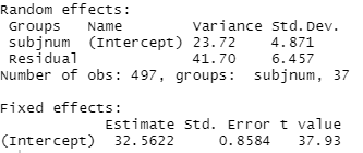
(a) Calculate and interpret the intraclass correlation coefficient
Model1
instructor = ifelse(musicians$audience == "Instructor", 1 , 0)
students = ifelse(musicians$audience == "Students", 1, 0)
summary(model1 <- lmer(pa ~ 1 + instructor + students + (1 + instructor + students | subjnum), data = musicians))
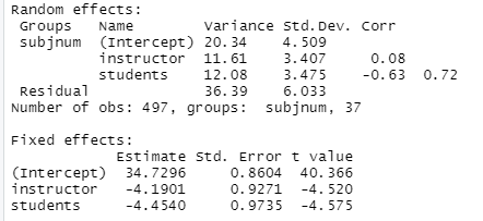
(b) Interpret the 34.73, -4.19, and 4.51 values in context.
(c) Calculate a (pseudo) R2 for Level 1 for this model.
Model2
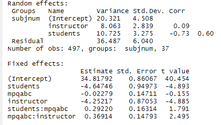
(d) Write the corresponding model out as Level 1 and Level 2 equations. (In terms of parameters, not estimates). How many parameters are estimated in this model?
(e) Provide interpretations for all estimated parameters!
(f) Which variance components decreased the most between Model1 and Model2? Provide a brief interpretation.
(g) Suppose I want to add an indicator variable for male to Model 2 as a predictor for all intercept and slope terms. How many parameters will this add to the model?
(h) Suppose I add the male indicator to Model 2 as suggested. How will this change the interpretations you gave in (e)?
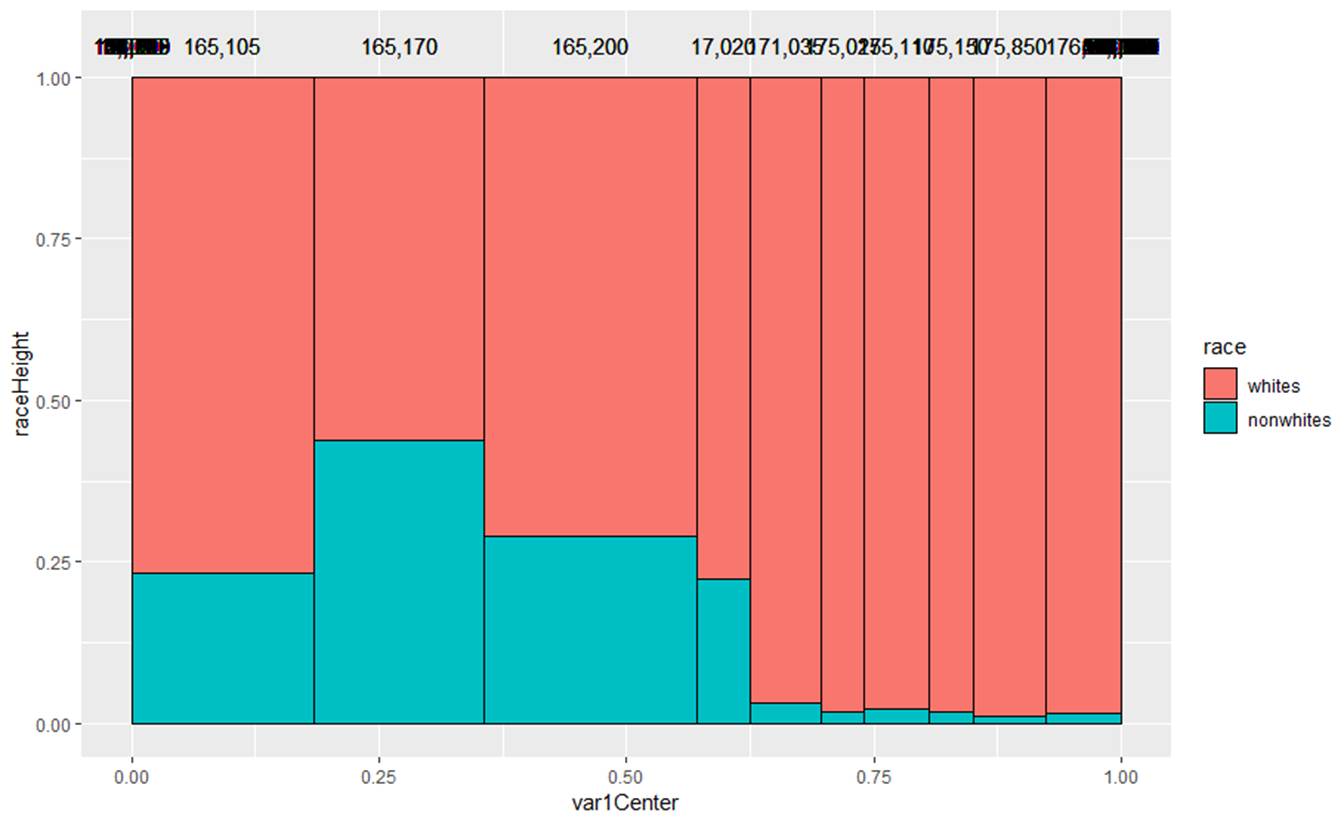
2) Kentucky Math Scores
Data were collected on 48,058 students from 235 middle schools from 132 different districts. These students were Kentucky eighth graders who took the California Basic Educational Skills Test in 2007. However, this analysis involves only 46,940 students who are complete cases. The variables of interests from this data set are:
- sch_id = School Identifier
- nonwhite = 1 if student is Not White and 0 if White
- mathn = California Test of Basic Skills Math Score
- sch_ses = School-Level Socio-Economic Status (Centered)
Main Objective: Is there a difference in math scores of eighth graders in Kentucky based on ethnicity and socioeconomic status, after accounting for the multilevel nature of the data?
(a) Summarize what you learn from the following graphs
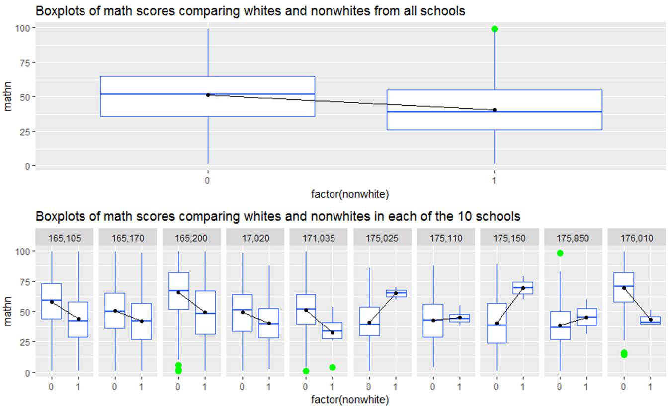
(b) Summarize what you learn from the following graph (for the same 10 schools)
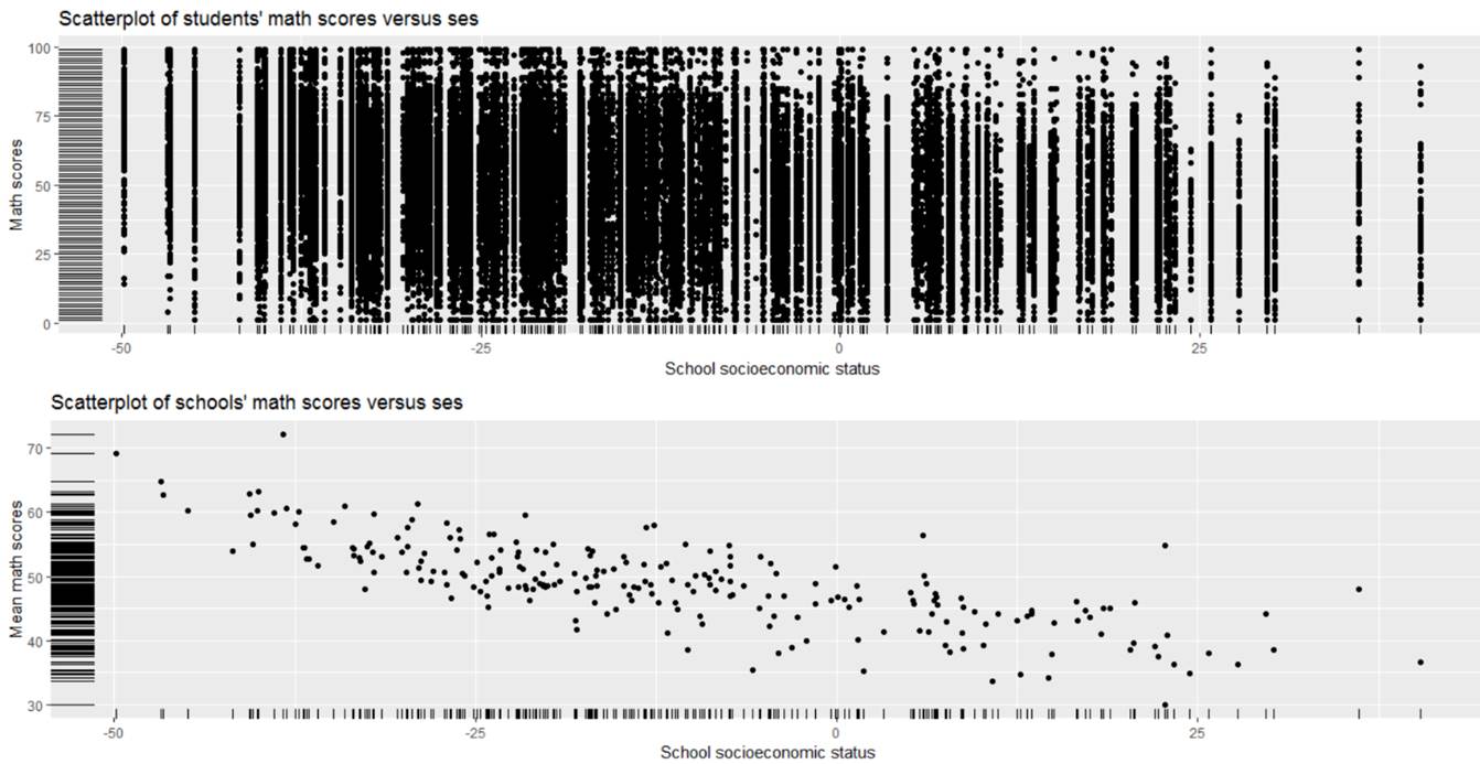
(c) Summarize what you learn from the following graphs
(d) For each school separately, I have run a traditional regression to predict math score from student race (1 = nonwhite, 0 = white). For each school, I saved the intercept and slope of that regression. Below are the results
|
|
> summary(intercepts) Min. 1st Qu. Median Mean 3rd Qu. Max. 31.0 45.9 49.8 50.1 54.3 77.4 > summary(slopes) Min. 1st Qu. Median Mean 3rd Qu. Max. NA's -34.190 -14.986 -8.610 -6.799 0.061 34.955 21
|
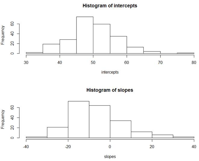
Briefly summarize what you learn.
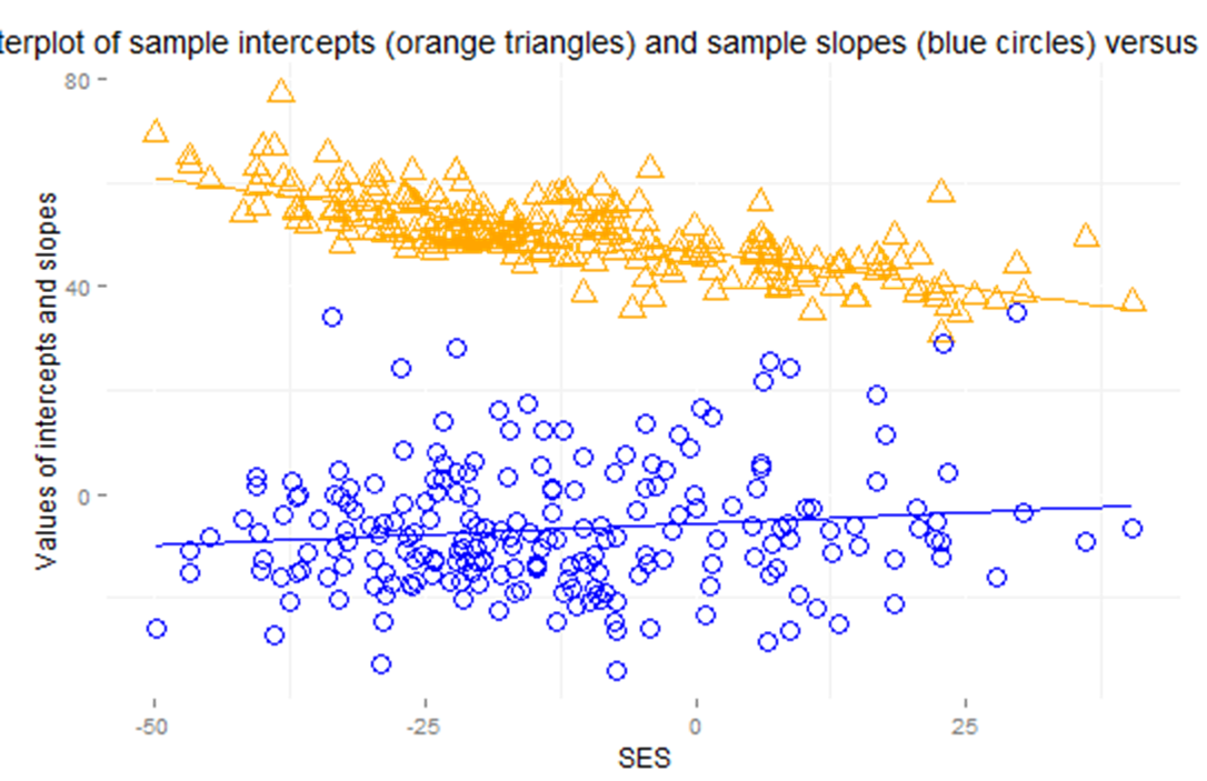
(e) Summarize, in context, what you learn about the association between the slopes and intercepts.
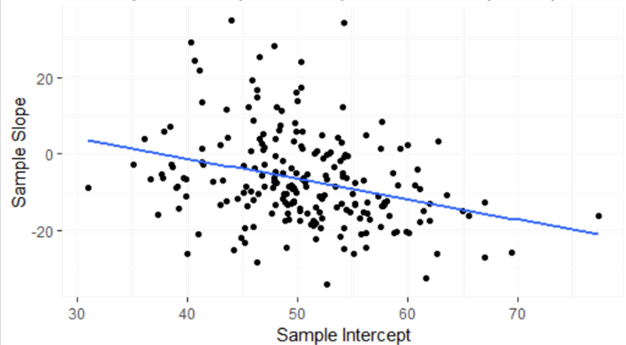
(f) Describe the nature of the association between ses and the sample intercepts and between ses and the sample slopes. Is there preliminary evidence that ses is a good predictor of the sample intercepts and sample slopes based on the associations? [Hint: What do these slopes represent?]
(g) Below is output from regressing the intercepts on the school SES and then from regressing the slopes on the school SES.
Summarize what you learn.
> model.intercept = lm(intercepts ~ mean.ses$x)
> summary(model.intercept)
Call:lm(formula = intercepts ~ mean.ses$x) Residuals: Min 1Q Median 3Q Max -13.112 -3.349 -0.659 2.549 19.742 Coefficients: Estimate Std. Error t value Pr(>|t|) (Intercept) 46.8675 0.3616 129.6 <2e-16 ***mean.ses$x -0.2811 0.0166 -16.9 <2e-16 ***---Signif. codes: 0 ‘***’ 0.001 ‘**’ 0.01 ‘*’ 0.05 ‘.’ 0.1 ‘ ’ 1 Residual standard error: 4.71 on 233 degrees of freedomMultiple R-squared: 0.551, Adjusted R-squared: 0.549 F-statistic: 286 on 1 and 233 DF, p-value: <2e-16
> model.slope = lm(slopes ~ mean.ses$x)
> summary(model.slope)
Call:
lm(formula = slopes ~ mean.ses$x)
Residuals:
Min 1Q Median 3Q Max
-27.86 -7.48 -1.97 7.55 42.78
Coefficients:
Estimate Std. Error t value Pr(>|t|)
(Intercept) -5.7084 1.0210 -5.59 0.000000069 ***
mean.ses$x 0.0847 0.0460 1.84 0.067 .
---
Signif. codes: 0 ‘***’ 0.001 ‘**’ 0.01 ‘*’ 0.05 ‘.’ 0.1 ‘ ’ 1
Residual standard error: 12.2 on 212 degrees of freedom
(21 observations deleted due to missingness)
Multiple R-squared: 0.0157, Adjusted R-squared: 0.0111
F-statistic: 3.39 on 1 and 212 DF, p-value: 0.0671
Is either association statistically significant? How much of the variation in intercepts and slopes is explained by the school SES?
(h) How do the above results compare to the “unconditional means” (null, random intercepts only) model?
> lmer(mathn ~ 1 + (1 | sch_id), REML=TRUE, data=math)
Linear mixed model fit by REML ['lmerMod']Formula: mathn ~ 1 + (1 | sch_id) Data: mathREML criterion at convergence: 416975Random effects: Groups Name Std.Dev. sch_id (Intercept) 6.32 Residual 20.40 Number of obs: 46940, groups: sch_id, 235Fixed Effects:(Intercept) 49
(i) Calculate and interpret the intraclass correlation coefficient.
(j) Below is the multilevel model version of the analysis.

Interpret each estimated parameter.
(k) Which predictors would you consider significant? Are the results consistent with what you learned in (g)? Explain.
(l) Below is a “one-level” analysis of the data, ignoring the school IDs.
> summary(lm(math$mathn ~ math$nonwhite + math$sch_ses + math$nonwhite:math$sch_ses))
Call:lm(formula = math$mathn ~ math$nonwhite + math$sch_ses + math$nonwhite:math$sch_ses) Residuals: Min 1Q Median 3Q Max -58.12 -14.48 0.39 14.14 65.96 Coefficients: Estimate Std. Error t value Pr(>|t|) (Intercept) 46.39809 0.13353 347.48 <2e-16 ***math$nonwhite -10.36714 0.40456 -25.63 <2e-16 ***math$sch_ses -0.30420 0.00562 -54.13 <2e-16 ***math$nonwhite:math$sch_ses 0.00984 0.01771 0.56 0.58 ---Signif. codes: 0 ‘***’ 0.001 ‘**’ 0.01 ‘*’ 0.05 ‘.’ 0.1 ‘ ’ 1 Residual standard error: 20.5 on 46936 degrees of freedomMultiple R-squared: 0.0881, Adjusted R-squared: 0.088 F-statistic: 1.51e+03 on 3 and 46936 DF, p-value: <2e-16
Do any of the conclusions change?
(m) Why do you think our conclusion about the significance of the SES x race interaction is so different between these two approaches?
3) Reconsider the NLSY data on children’s anti-social behavior (measured in 1990, 1992, 1994) as the response variable, with
· self = self-esteem, measured with a scale ranging from 6 to 24
· pov = poverty status of family, coded 1 for in poverty, 0 otherwise
time-varying variables. Time invariant variables include child’s age at start of study, mom’s age at birth etc.
(a) Suppose we fit an ordinary least squares (OLS) regression to the data.
What do we consider to be the main flaw in this analysis? What do we expect to be the main consequence of this flaw? Interpret the coefficient of poverty in this model. Does poverty appear to be a statistically significant predictor of anti-social behavior?
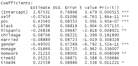
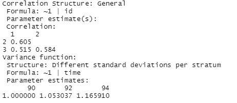
(b) Suppose we fit the following model:
model1a = gls(anti ~ self + pov + black + hispanic + childage + married + gender + momage + momwork + time, corr = corSymm(form = ~ 1 | id), weights = varIdent(form = ~1 | time), method="ML", data = nlsy_long)
![]()
Explain what the parameter estimates of 0.605, 0.515, and 0.584 represent. Explain what the parameter estimates of 1.00, 1.05, and 1.165 represent. (What were some of your clues in the output/R command to help you understand the model being fit?) How many total parameters are estimated in this model?
Bonus question: what will the variance-covariance matrix for this model look like? How will it compare to the same matrix in (a)? How many parameters are estimated?
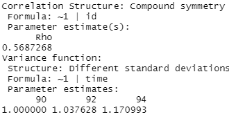
(c) Suppose we fit the following model
model2a = gls(anti ~ self + pov + black + hispanic + childage + married + gender + momage + momwork + time, corr = corCompSymm(form = ~ 1 | id), weights = varIdent(form = ~1 | time), method="ML", data = nlsy_long)
![]()
Explain the model implications.
Bonus question: what will the variance-covariance matrix for this model look like? How will it compare to the others? How many parameters are estimated?
(d) Suppose we fit the following model:
model3 = lme(anti ~ self + pov + black + hispanic + childage + married + gender + momage + momwork + year, random = ~1 | id, method= "ML", data = nlsy_long)

What is the intraclass correlation coefficient? What does the variance-covariance matrix for this model look like? Is there more variation at Level 1 or Level 2 in this data? Does that make sense?
(e) The model in (c) matches what we get from the random intercepts model for the correlation matrix for the model in (d), but the random intercept model in (d) assumes equal variances. How would I adjust the multilevel model in (d) to allow for unequal variances?
(f) The resulting standard errors from the multilevel model (from d) are considered more valid.
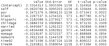
How do these standard errors compare to the ols model? Does poverty appear to be a statistically significant predictor of anti-social behavior?
The “fixed” model below includes the children id in the model as a fixed effect. This adjusts the standard errors for dependence and controls for all stable characteristics of the individuals.
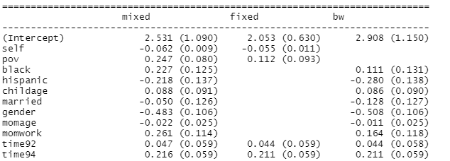
(g) The fixed effects model does not include any Level 2 variables. Why not? (Though we could include interactions with level 2 variables.)
(h) This noticeably changes the poverty coefficient. How would you now interpret the coefficient? How has the standard error for poverty changed?
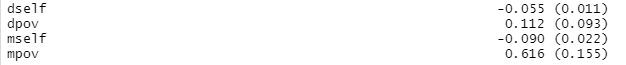
We discussed the “Hausman test” before as a comparison of these two models to see whether the mixed effects model (random effects) adequately accounts for all important potential Level 2 variables (no confounding between a Level 1 variable and something at the group level.) A hybrid approach is called a “between-within” model (bw). The bw model is again just our mixed model with both level 1 (deviation) and level 2 variables (group mean).
(i) How does the coefficient of poverty compare between the 3 models? (Hint: Which is it equal to and why?)
(j) Does there appear to be a practical and/or significant difference between the “within” effect of poverty and the “between” effect of poverty? How are you deciding? Which is worse, changing poverty status or being a person in poverty?
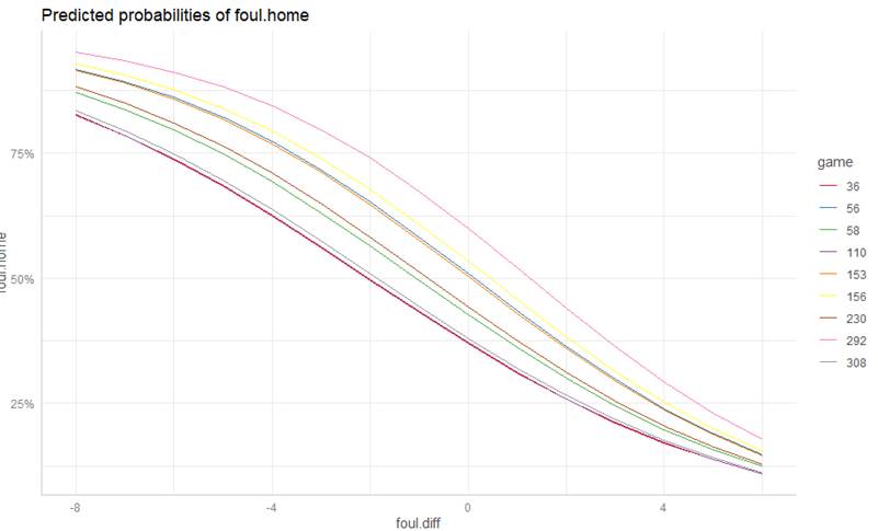
4) An article by K. J. Anderson and Pierce (2009) describes empirical evidence that officials in NCAA men’s college basketball tend to “even out” foul calls over the course of a game, based on data collected in 2004-2005. Using logistic regression to model the effect of foul differential on the probability that the next foul called would be on the home team (controlling for score differential, conference, and whether or not the home team had the lead), they found that “the probability of the next foul being called on the visiting team can reach as high as 0.70.” More recently, Moskowitz and Wertheim (2011), in their book Scorecasting, argue that the number one reason for the home field advantage in sports is referee bias. Specifically, in basketball, they demonstrate that calls over which referees have greater control—offensive fouls, loose ball fouls, ambiguous turnovers such as palming and traveling—were more likely to benefit the home team than more clear-cut calls, especially in crucial situations. In this exercise, you will examine data collected by Noecker and Roback from the 2009-2010 basketball season for the first half of 340 games in the Big Ten, ACC, and Big East conferences. The basketball0910.txt data file has a row for each of 4,972 fouls. The primary response variable is foul.home, 1 if the foul was called on the home team. The hypothesis is that if more fouls have been called on the home team than the visiting team, the probability is smaller that the next foul is on the home team.
bball = read_delim("http://rossmanchance.com/stat414/data/basketball0910.txt", "\t", escape_double = FALSE, trim_ws = TRUE)
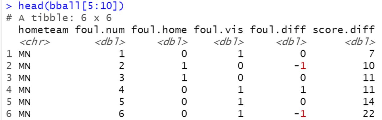
When a foul is called, we keep track of whether it was called on the home team or the visitor team. foul.diff shows the difference in the number of fouls called so far on the home team rather than the visiting team. In row 1, the foul is called on the visitor, so in row 2, foul.diff = -1. In row 2, the foul is called on the home team, so in row 3, the difference is zero. In row 3, the foul is called on the home team again, so now they have had one more foul called on them and foul diff in the next row is 1.
We plan to fit a multilevel logistic model including random slopes for the foul differential:
summary(glmer(foul.home ~ foul.diff + (foul.diff | game), family = binomial, data = bball) )
(a) Write out the Level 1 and Level 2 equations, including variance/covariance components.
(b) Interpret the sign of the foul.diff slope. Does it support the conjecture?
> summary(glmer(foul.home ~ foul.diff + (foul.diff | game), family = binomial, data = bball) )
|
boundary (singular) fit: see ?isSingular Generalized linear mixed model fit by maximum likelihood (Laplace Approximation) [glmerMod] Family: binomial ( logit ) Formula: foul.home ~ foul.diff + (foul.diff | game) Data: bball
AIC BIC logLik deviance df.resid 6791.1 6823.6 -3390.5 6781.1 4967
Random effects: Groups Name Variance Std.Dev. Corr game (Intercept) 0.294145 0.54235 foul.diff 0.001235 0.03514 -1.00 Number of obs: 4972, groups: game, 340
Fixed effects: Estimate Std. Error z value Pr(>|z|) (Intercept) -0.15684 0.04637 -3.382 0.000719 *** foul.diff -0.28533 0.03835 -7.440 1.01e-13 *** |
|
(c) Now consider the following model with crossed random effects
> summary(model3 <- glmer(foul.home ~ foul.diff + (1 | game) + (1 | hometeam) + (1 | visitor), family = binomial, data = bball) )
Generalized linear mixed model fit by maximum likelihood (Laplace
Approximation) [glmerMod]
Family: binomial ( logit )
Formula:
foul.home ~ foul.diff + (1 | game) + (1 | hometeam) + (1 | visitor)
Data: bball
AIC BIC logLik deviance df.resid
6780.5 6813.0 -3385.2 6770.5 4967
Scaled residuals:
Min 1Q Median 3Q Max
-1.6589 -0.9056 -0.6522 0.9679 1.7952
Random effects:
Groups Name Variance Std.Dev.
game (Intercept) 0.17165 0.4143
hometeam (Intercept) 0.06809 0.2609
visitor (Intercept) 0.02323 0.1524
Number of obs: 4972, groups: game, 340; hometeam, 39; visitor, 39
Fixed effects:
Estimate Std. Error z value Pr(>|z|)
(Intercept) -0.18780 0.06331 -2.967 0.00301 **
foul.diff -0.26385 0.03883 -6.795 1.08e-11 ***
Now consider a model that accounts for score differential, whether the home team has the lead, time left in the first half, type of foul, the interaction between foul differential and type of foul, the interaction between foul differential and time, and the interaction between home team lead and time, with random intercepts for game, home team, and visiting team.
summary(model5 <- glmer(foul.home ~ foul.diff + score.diff + lead.home +
time + foul.type + foul.diff:foul.type + foul.diff:time + lead.home:time + (1 | game) + (1 | hometeam) + (1 | visitor), family = binomial, data = bball))
exp(fixef(model5))
Fixed effects:
Estimate Std. Error z value Pr(>|z|)
(Intercept) -0.328087 0.157636 -2.081 0.03741 *
foul.diff -0.274966 0.062215 -4.420 9.89e-06 ***
score.diff 0.033515 0.008236 4.069 4.72e-05 ***
lead.home -0.150126 0.177231 -0.847 0.39696
time -0.008693 0.008561 -1.015 0.30992
foul.typePersonal 0.148216 0.108605 1.365 0.17234
foul.typeShooting 0.081163 0.111237 0.730 0.46561
foul.diff:foul.typePersonal 0.047689 0.052306 0.912 0.36191
foul.diff:foul.typeShooting 0.103333 0.053867 1.918 0.05507 .
foul.diff:time -0.008700 0.003274 -2.657 0.00788 **
lead.home:time 0.025947 0.012173 2.132 0.03304 *
(e) Summarize the signs of the coefficients of the interactions.
Curran, Stice, and Chassin (Journal of Consulting and Clinical Psychology, 1997) collected data on 82 adolescents at three time points starting at age 14 to assess factors that affect teen drinking behavior. Key columns in the data set are:
· id = numerical identifier for subject
· age = 14, 15, or 16
· coa = 1 if the teen is a child of an alcoholic parent; 0 otherwise
· male = 1 if male; 0 if female
· peer = a measure of peer alcohol use, taken when each subject was 14. This is the square root of the sum of two 6-point items about the proportion of friends who drink occasionally or regularly.
· alcuse = the primary response. Four items—(a) drank beer or wine, (b) drank hard liquor, (c) 5 or more drinks in a row, and (d) got drunk—were each scored on an 8-point scale, from 0=“not at all” to 7=“every day.” Then alcuse is the square root of the sum of these four items.
Primary research questions included:
· Do trajectories of alcohol use differ by parental alcoholism?
· Do trajectories of alcohol use differ by peer alcohol use?
(a) Identify Level One and Level Two predictors.
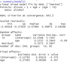
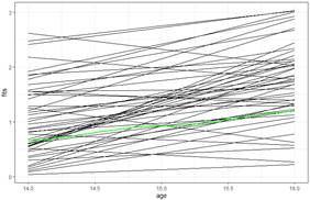
(b) Run an unconditional growth model with age as the time variable at Level One. (include time and random slopes for time) Interpret the intercept.
model1 = lmer(alcuse ~ 1 + age + (1 + age | id), data = alcohol)
(c) Create age14 = age-14. Explain the advantage of doing so.
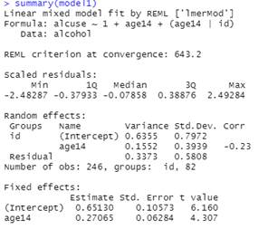
(d) Rerun the unconditional growth model using age14, how do things change? (model1) Calculate and interpret an R2 value for the Level 1 variance comparing this model to the null model.
model1 = lmer(alcuse ~ 1 + age14 + (1 + age14 | id), data = alcohol)
(e) Add the effects of having an alcoholic parent and peer alcohol use in both Level Two equations to model 1.
|
|
|
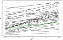
Report and interpret all estimated fixed effects, using proper notation (Think about what the graphs will look like)
This is my attempt to have you come up with the models
6) Chapp et al. (2018) explored 2014 congressional candidates’ ambiguity on political issues in their paper, Going Vague: Ambiguity and Avoidance in Online Political Messaging. They hand coded a random sample of 2012 congressional candidates’ websites, assigning an ambiguity score. These 2014 websites were then automatically scored using Wordscores, a program designed for political textual analysis. In their paper, they fit a multilevel model of candidates’ ambiguities with predictors at both the candidate and district levels.
Variables of interest include:
· ambiguity = assigned ambiguity score. Higher scores indicate greater clarity (less ambiguity)
· democrat = 1 if a Democrat, 0 otherwise (Republican)
· incumbent = 1 if an incumbent, 0 otherwise
· ideology = a measure of the candidate’s left-right orientation. Higher (positive) scores indicate more conservative candidates and lower (negative) scores indicate more liberal candidates.
· mismatch = the distance between the candidate’s ideology and the district’s ideology (candidate ideology scores were regressed against district ideology scores; mismatch values represent the absolute value of the residual associated with each candidate)
· distID = the congressional district’s unique ID (Level 2 units)
(a) Is ideological distance [from district residents] associated with greater ambiguity, but to varying degrees across the districts?
(b) Does the impact of ideological distance depend on the attitudinal heterogeneity among voters in the district?
(c) Controlling for ideological distance, does ideological extremity [of the candidate] correspond to less ambiguity?
(d) Does more variance in attitudes [among district residents] correspond to a higher degree of ambiguity in rhetoric?
(e) Does candidate rhetoric become clearer as the candidate’s issue positions move to the ideological extremes?
(f) Does the variability in ambiguity scores differ for Republican and Democratic candidates?