Stat 414 – HW 1
Due by midnight, Friday, Sept. 29
This first assignment does assume you remember a few topics from earlier courses, like interpreting the regression equation, interpreting R2, transformations, etc. You may need to continue reviewing your notes from your previous courses, be sure to ask questions! Cite your sources!
Please submit problems 2-5 as
separate files in Canvas (doc or pdf format)
1)
Introductions/Initial Surveys
2) For each study (a)-(c) below
(i)
Identify the Level 1
units
(ii)
Identify the
response variable and at least one explanatory variable(s)
(iii)
Translate the LINE
assumptions for inference in the context of the study
(iv)
Comment on whether
each assumption is likely to be met, or identify which
assumption you think is most suspect and why.
These
questions are open to interpretation so be sure to explain your reasoning!
(a) Do wealthy families tend to have fewer children compared to lower income
families? Annual income and family size are recorded for a random sample of
families.
(b) The yield
of wheat per acre for the month of July is thought to be related to the
rainfall. A researcher randomly selects acres of wheat and records the rainfall
and bushels of wheat per acre.
(c) Medical
researchers investigated the outcome of a particular surgery for patients with
comparable stages of disease but different ages. Each of the ten hospitals in
the study had at least two surgeons performing the surgery of interest.
Patients were randomly selected for each surgeon at each hospital. The surgery
outcome was recorded on a scale of one to ten.
3) Following up on the Kentucky Derby data we examined this week. Most of the time the track condition is listed as “fast” (rather than slow or muddy etc.).
(a) With the KYDerby23 dataset, execute the following command and explain what it does (provide supporting evidence for your discussion).
fast = ifelse(KYDerby23$condition == "fast", "fast", "notfast")
[Note: You can often copy and paste commands into R, but watch out for things like capitalization and “curly quotes”]
(b) With a binary explanatory variable, we can carry out a two-sample t-test. In R:
t.test(KYDerby23$speed ~ fast)
Include your output. What is the observed difference in
means? Report the t-statistic
and two-sided p-value.
(c) With a binary
explanatory variable, we can also fit a regression model:
summary(lm(KYDerby23$speed ~ fast))
Include your output. Is
R using “indicator” coding or “effect” coding? How can you tell? What does the
slope of this line tell you?
(d) Are the
p-values in (b) and (c) equal? Why not?
(Hint: What are the assumptions between the two models?)
(e) Include output for summary(aov(KYDerby23$speed ~ fast)). Is this analysis equivalent to either (b) or (c)? Explain as if to someone wondering which analysis to use.
(f) From your output in (c), what is the “standard error of the slope” value? Write a one-sentence interpretation of this value and of the t-statistic for the slope. If you only knew the t-statistic value, would you have considered the relationship statistically significant? Explain your reasoning.
4) A British study (North, Shilcock, & Hargreaves, 2003) examined whether the type of background music playing in a restaurant affected the amount of money that diners spent on their meals. The researchers asked a restaurant to alternate classical music, popular music, and silence on successive nights over 18 days. The following summary statistics about the total bills were reported:
|
|
Classical music |
Pop music |
No Music |
|
|
Mean |
£24.13 |
£21.91 |
£21.70 |
|
|
SD |
£2.243 |
£2.627 |
£3.332 |
|
|
Sample size |
n1 = 120 |
n2 = 142 |
n3 = 131 |
n = 393 |
(a) State the null and alternative hypotheses corresponding to the researchers’ conjecture (in symbols and/or in words, be sure to define any symbols you use).
(b) Based on these summary statistics, calculate the overall (weighted) mean tip amount, the between group variation, and the pooled variance. Check the consistency of your calculations with the summary statistics. (Show your work!)
Overall
(weighted) mean: ![]()
Between
group variability (MSGroups) = ![]()
Pooled variance
(MSError) = 
Explain in your own words what the last quantity measures.
(c) Use your calculations in (b) to calculate the F-statistic for the hypotheses in (a). Would you consider this F-statistic statistically significant? Explain.
(d) In F Probability Calculator applet: Specify the degrees of freedom and the observed F-value, and the direction for the probability of interest. What do you conclude from this p-value?
(e) Suppose the between group variability is larger, would the F-statistic be larger or smaller? Suppose the pooled standard deviation was smaller, would the F-statistic be larger or smaller?
(f) Explain why the
analysis you have carried out is invalid for these data.
5) Suppose that you are interested in purchasing a used car. How much should you expect to pay?
(a) Identify 2 variables that you believe would be very useful in estimating the price of the car. Are these variables generally available to you?
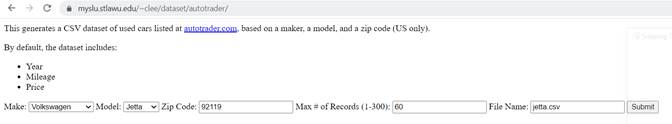
(b) To get a sample lots of cars, go to the webpage https://myslu.stlawu.edu/~clee/dataset/autotrader/ which will obtain data from listings at autotrader.com. Pick a car make and model (e.g., Honda Accord) and a zip code to sample from (e.g., your home town?). You eventually want a sample of 50 used cars, so ask for 60 or so to start in case you need to do some pruning. Also, choose a name for the dataset with a .csv extension.
If you have trouble getting a large enough sample, try a different zip code (e.g., LA or SF).
(c) After saving your data, check the spreadsheet to see whether some cases should be deleted. What are some reasons you would delete a case? Do you need to delete any?
(d) What are the measurement units for price and mileage? (If you aren’t sure, ask).
(e) In Excel or Google sheets, create a new variable called age, for example,
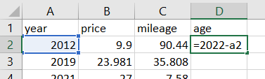
(and then double click on the square in the lower right corner to fill down).
(f) Get the data into R (Try using cars = read.table("clipboard", header=T) to load the data into R?) and include a histogram of the prices. What is the standard deviation of the prices?
(g)
Create a scatterplot and find the correlation coefficient cor(x,y) between price and age. Include your output
and summarize the behavior of the relationship between price and age.
Extra
credit: Consider something
like psych::scatter.hist(cars$age,
cars$price, xlab="age",
ylab="price", smooth=F, ab =T, ellipse =
F) from the psych package
(h) Fit a regression model to predict price from age. Write out the regression equation using good statistical notation. Interpret the intercept and slope coefficients in context.
(i) What is the standard error of the residuals from your R
output, ![]() ?
Compute
?
Compute ![]() . How does this value compare to R2?
Extra Credit: Why aren’t they exactly the same?
. How does this value compare to R2?
Extra Credit: Why aren’t they exactly the same?
(j) Produce (and include) a graph of residuals vs. fitted values. Explain what you learn from this graph.
(k) Does the normality assumption appear to be met? Clearly explain how you are deciding.
(l) Fit a quadratic model. Describe the “implications” of this equation – what does it tell you about the behavior of price vs. age. Does this behavior make sense in this context? Explain.
Not graded: (m) Fit a model to predict price from age and mileage. Now how do you interpret the coefficient of age? Be very clear how your interpretation changes from (h).