Stat 301 - HW 8

Due midnight, Friday, March 15

Remember to put your names in this file and to include and integrate all relevant computer output.

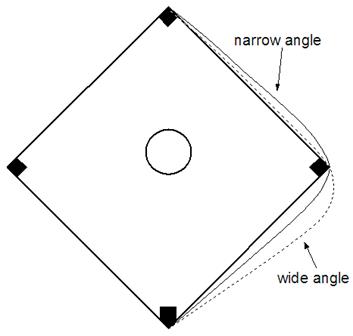
1) In baseball, when running from say home plate to second base, does the path that you take to “round” first base make much of a difference? Hollander and Wolfe (1999) report on a Master’s Thesis by W. F. Woodward (1970) that investigated different base running strategies. For example, you could take a “narrow angle” or a “wide angle” around first base.

In Woodward’s study, he planned to use a stopwatch to time runners going from a spot 35 feet past home to a spot 15 feet before second based. He had access to 22 different runners. Woodard wanted to test H₀: m_narrow - m_wide = 0 vs. H_a: m_narrow - m_wide ≠ 0.

(a) Suppose he tells you that the standard deviation of running speeds among such runners is about 0.30 seconds. Give a one-sentence interpretation of this value.

(b) According to somatechnology.com, the average human eye blink is 0.10 seconds. If Woodward randomly assigns these 22 runners to two groups of 11, use the Normal Probability Calculator applet (or R’s pnorm and qnorm functions or iscaminvnorm and iscamnormprob) to approximate the power he will detect a difference in mean running time in a two-sided test:

Step 1: Assume a normal distribution for the difference in sample means with mean 0 and standard deviation

Step 2: Find the times that correspond to the 97.5^th and 2.5^th percentiles of this distribution.

Include a screen capture of your results.

Step 3: Now assume a normal distribution for the difference in sample means with mean 0.10 and standard deviation 0.1279.

Include a screen capture of your results.

What is the probability that Woodard will correctly reject the null hypothesis in this case?

(c) Instead, Woodward conducted a paired-design with his 22 runners, asking each runner to use each method, with a rest period in between, randomizing which method they used first. Should the variability in the time differences be larger or smaller than the variability in the times? Explain your reasoning.

(d) Suppose the variability in the time differences is 0.10. Calculate the power that he would detect a nonzero mean difference in running time in a two-sided test. (Repeat the two-step process in (b), first estimating the standard error, including both relevant screen captures. Also include a one-sentence interpretation of this power, in context. How do the power calculations compare?

The data in BaseRunning.txt shows the time (in seconds) for each running using the narrow angle and the wide angle. His original hypotheses are equivalent to testing H₀: m_diff = 0 vs. H_a: m_diff ≠ 0.

(e) Carry out a simulation analysis of the paired data using the Matched Pairs applet (the data are preloaded into the applet). Include a short description of the simulation process and what it represents. Include a screen capture of the simulated null distribution with the two-sided p-value.

(f) Use R or the Applet to carry out the one-sample t-test on the differences (aka a matched-pairs t-test). Note: R allows you to use the “unstacked” format of these data.

R br <- read.delim("http://www.rossmanchance.com/iscam3/data/BaseRunning.txt", sep="\t") t.test(br$wide, br$narrow, paired=TRUE)

Applet Change the statistic to t-statistic Enter the observed t-statistic in the Count Samples box and check the Overlay t box.

Include a screen capture of the results and report the test statistic and two-sided p-value.

(g) Does the t-test appear to be valid for these data? You should comment on the validity conditions of the paired t-test as well as how the results in (e) and (f) compare.

(h) Carry out a sign test on the paired data:

1. Calculate the time differences (narrow – wide) (You can use the dotplot in the applet.)

2. How many of the differences are positive? How many are negative? How many are zero?

3. Consider the non-zero differences, what proportion are positive?

4. Use the binomial distribution to determine whether there is a statistically significant majority of the differences are positive (define the parameter of interest, state the hypotheses, and determine the exact binomial p-value – be sure to include a screen capture)

(i) Does the sign test provide stronger or weaker evidence that one base-running method tends to be faster than the other? (Note: You should compare the two-sided p-values to each other.)

(j) Would a one-sample z-test be appropriate in (h)? Explain how you are deciding.

(k) Determine, include, and interpret in context a 95% confidence interval for . This time, consider your answer to (j) in deciding which interval procedure to use.

2) Based on your responses to Question 4 on HW 7, I have created two datasets:

short.txt

long.txt

containing your original water usage value and your “realistic” adjusted water usage value, depending on whether you were using the short form or the long form.

Use R or the Matched Pairs applet.

(a) Examine the data with the short form. One observation stands out to me as unusual. What graph did you look at to spot it? I believe there is an error in the data reported – what do you think happened? (Hint: See (c) as well?)

(b) Remove the unusual observation in (a) (document how you do so, you can replace a value with * or remove both observations and reload the data?) and provide a dotplot and numerical summaries for the differences between the original and adjusted values. Also produce and interpret a 95% t-confidence interval using the differences. Include your output.

(c) Now consider the data from the long form. Again we have one strange observation, perhaps with the same explanation? Remove this observation and produce numerical and graphical summaries of the differences. Produce a t-confidence interval and discuss the similarities and differences compared to the interval in (b). Include your output!

Reminder: Course Evaluations due Friday night as well!