Stat 301 - HW 6

Due midnight, Friday, Feb. 23

Remember to put your name(s) inside each file and, if submitting together, join a HW group first. Remember to show your work/calculations/computer details and to integrate this into the body of the solution.

1) The common wart typically resolves itself without treatment within 2 years. However, many patients request treatment to speed up this process. Focht, Spicer, and Fairchock (Arch Pediatr Adolesc Med. 2002) compared the standard treatment (cryotherapy with liquid nitrogen, which can be painful and scary for children) to tape occlusion therapy (using adhesive tape for 6.5 days, removing for 12 hours, and then repeating; painless and inexpensive). They conducted a “conducted a prospective, randomized trial of duct tape occlusion therapy vs our local standard of cryotherapy in the treatment of common pediatric warts“ to see if the duct tape would lead to a higher cure rate. A patient was considered “cured” there was complete resolution of the wart being studied within 2 months.

A close up of a text

Description automatically generated

Patients aged 3 to 22 years were randomized to cryotherapy or duct tape. Of the 61 patients enrolled, 51 completed the study. Here are their results:

	Cryotherapy	Duct Tape	Total
Cured	15	22	37
Not cured	10	4	14
Total	25	26	51

(a) Identify the observational units, explanatory variable, and response variable for this study. Which response variable outcome will you consider “success”?

(b) Was this study observational or experimental? Explain how you are deciding.

(d) State appropriate null and alternative hypotheses for determining whether the duct therapy would be more effective than the cryotherapy in curing the common wart.

(e) Use the Two-way Tables applet to enter the data.

· Check the Enter table box. Enter the appropriate counts, as well as short (one-word) column and row names.

o Note: the applet allows you to enter in the subtraction expression to find the number of “failures.”

o Be sure to press Use Table when you are done.

· Check the Show Table box and include a screen capture of the graph (either a bar graph or mosaic plot) and the observed two-way table.

Write a one-sentence interpretation of the statistic. Does the statistic provide preliminary evidence in favor of the researcher’s claim that tape occlusion is more effective than cryotherapy?

(f) Use the applet to carry out a simulation-based randomization test for the difference in conditional proportions:

· Check the Show Shuffle Options box.

· Enter a large number of shuffles and press Shuffle.

· Use the Count Samples box (and appropriate direction) to find the simulation-based p-value and press Count.

· Include a screen capture of your null distribution, with the p-value displayed.

Summarize the conclusion you would draw about this research question, in context, based on this p-value. Are you willing to draw a cause-and effect conclusion from this study? Explain why or why not. To what population are you willing to generalize these results? Justify your choice.

(g) Use the applet to find the “exact p-value”

· Check the Show Fisher’s Exact Test p-value box.

· What values of k, N, M, and n are being used for this hypergeometric probability calculation?

How do the exact and simulation-based p-values compare? Is this what you expected?

(h) Find the two-sample proportion z-test p-value.

· Check the Overlay normal distribution p-value.

How do the exact and normal-based p-values compare? Is this what you expected? (Clearly explain what you expected and why.)

(i) Suggest a strategy for improving this approximation of the p-value and roughly carry out this strategy by using your mouse to move the red “count line.” Don’t worry about being too precise here, just explain the process. Include a screen capture of your null distribution and new p-value estimate.

(j) Determine the two-sample proportion z interval with the “Wilson adjustment”:

· Add 1 success and 1 failure to each treatment and press Use Table.

· Check the 95% CI(s) for difference in proportions box on the left

· Include a screen capture of your results.

Interpret your interval in context, being sure to indicate “direction.”

(k) Explore the relative risk statistic:

· Change the counts back to the observed values (and press Use Table).

· Use (either) Statistic pull-down menu to change the statistic to the relative risk (Option: Click on the GroupA/GroupB button to interchange the groups)

Include a one-sentence interpretation of the relative risk in context.

(l) Use the applet to carry out a simulation-based randomization test for the relative risk:

· Include a screen capture of your null distribution, with the p-value displayed.

How did the p-value change when you changed the statistic?

(m) Check the box for ln relative risk (on the left). Include a screen capture of the new null distribution. (You can clear the count box and press enter to make it rescale.) Is the distribution more symmetric? Based on this graph, why might the normal approximation still be a little risky?

(n) Use the formula from investigation 3.8 to approximate the standard deviation for the ln relative risk.

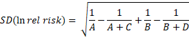
Show your work. How does this theoretical SD compare to your simulation results? (Be very clear what two numbers you are comparing.)

(o) Determine a 95% confidence interval for the relative risk

· Check the 95% CI for relative risk box on the left.

Interpret your interval in context, being sure to indicate “direction.”

(p) What interesting value is inside your confidence interval? Is this consistent with your p-value? Explain any discrepancies.

(q) Is the relative risk an appropriate statistic for this study? Explain your reasoning (e.g., it was not for the Wynder & Graham study).

2) Recall the studies on smoking and lung cancer from the 1950s (Investigation 3.10). Another landmark study on smoking began in 1952 (Hammond and Horn, 1958, “Smoking and death rates—Report on forty-four months of follow-up of 187,783 men: II. Death rates by cause,” JAMA). They used 22,000 American Cancer Society volunteers as interviewers. Each interviewer was to ask 10 healthy white men between the ages of 50 and 69 to complete a questionnaire on smoking habits. Each year during the 44-month follow-up, the interviewer reported whether or not the man had died, and if so, how. They ended up tracking 187,783 men in nine states (CA, IL, IA, MI, MN, NJ, NY, PA, WI). Almost 188,000 were followed up by the volunteers through October 1955, during which time about 11,870 of the men had died, 488 from lung cancer. The following table classifies the men as having a history of regular cigarette smoking or not and whether or not they died from lung cancer. In this study, nonsmokers are grouped with occasional smokers, including pipe- and cigar-only smokers.

Hammond and Horn	Not regular smoker	Regular smoker	Total
Lung cancer death	51	397	448
Alive or other cause of death	108,778	78,557	187,335
Total	108,829	78,954	187,783

(a) Is this a case-control, cohort, or cross-classified study? Explain your reasoning.

A third study (Wynder and Cornfield, 1953, “Cancer of the Lung in Physicians”, NEJM) examined physicians, believing they would be “homogenous economically, with little occupational exposure to respiratory irritants and with equal access to diagnostic facilities.” The researchers used death notices in the Journal of the American Medical Association in 1950 and 1951 to identify physicians who had died from various types of cancer. Letters were sent to the estates of those individuals to ask about their smoking status and type of cancer. The table below summarizes the responses.

	Wynder and Cornfield	Nonsmoker	Smoker	Total
Lung cancer patient		3	60	63
Other cancer		11	32	43
Total		14	92	106

(b) Is this study design best classified as case-control, cohort, or cross-classified? Explain your reasoning.

(d) Suggest one disadvantage to this study design compared to the Wynder & Graham and Hammond & Horn studies.

(e) Which of the three studies shows the strongest association between smoking status and lung cancer status? (You can treat the response variables as essentially the same across the 3 studies.) Support your answer numerically.

3) A study (reported in Julious & Mullee, 1994) compared two types of procedures for removing kidney stones: open surgery and percutaneous nephrolithotomy (PN), a “keyhole” surgery that removes the stone through the skin, designed to have much less disturbance than an open operation. In this study,

· For stones less than 2 cm, 81 of 87 cases of open surgery were successful compared to 234 of 270 cases of PN.

· For stone at least 2 cm, 192 of 263 cases of open surgery were successful compared to 55 of 80 cases of PN.

(a) Calculate the odds of success for stones less than 2cm with open surgery.

(b) Calculate the odds of success for stones less than 2cm with PN.

(d) Calculate and interpret in context, the odds ratio of success for stones at least 2 cm, comparing PN surgery to pen surgery.

(e) Create the two-way table using surgery outcome and type of procedure.

(f) From your table in (e), calculate the odds ratio of success comparing PN surgery to open surgery. How does this value compare to what you found in (c) and (d)? How would you explain this “paradox” to a non-statistician? (What is causing it? You might want to look at the three two-way tables next to each other and also the conditional proportions in each table.)

(g) Which type of surgery would you recommend? Explain.