Stat 301 - HW 5

Due midnight, Friday, Feb. 16

Please upload separate files for each problem and to put your name inside each file. Remember to show your work/calculations/computer details and to integrate this into the body of the solution. INCLUDE ALL RELEVANT OUTPUT.

R Users: You have the option of using the supplied RMarkdown file for problems 2 and 3.  Click on the file and open it in RStudio (or copy and paste the contents into a New File > R Markdown).  When you are done, press the Knit button.  I prefer you knit to Word or PDF. If you knit to Word, you have the option of adding the discussion in Word (and other cleanup!) rather than in the markdown file.  Submit only Word or PDF files. You can run lines individually and preview the result.  Remember that error messages apply to the entire chunk, not just the suggested line.

1) Complete the Stat 301 Midquarter Evaluation form in Canvas

2) I asked both sections to the complete a water usage journal and then submit the results from the water usage calculator. The results for 68 students are here. Define as the population mean water usage across all California college students.

Load the data into R or use hw5RMarkdown_2.Rmd. 

OR you can also use the Theory-Based Inference applet. Copy the data to your clipboard and then in the applet set the Scenario to One mean. Check the Paste data box and check the Includes header box. Paste the data into the data window, replacing the default data. Press Use Data.

(a) Create a well-labeled dotplot or histogram of the results. Summarize the shape, center, and variability of the distribution in context. Do you have any conjectures for any unusual features to this distribution?

(b) Discuss whether you think a one-sample t-procedure is valid for these data.

(c) Even if you said “no” in (b), calculate a one-sample t-confidence interval. Interpret your interval in context.

(d) The online water usage calculator you were provided included a national average of 1744. Does this seem to be a plausible value for based on these data? Explain your reasoning based on your interval in (c).

(e) Discuss whether you think a one-sample t-prediction is valid for these data.

(f) Even if you said “no” in (e), calculate a one-sample t-prediction interval. Interpret your interval in context. (If by hand, show your work!)

(g) How do the intervals in (c) and (f) compare (midpoint, width)? Is this what you expected? Explain.

An alternative approach to a t-confidence interval when you think the validity conditions are suspect is bootstrapping. Bootstrapping is most helpful when the t-procedures are not expected to be valid, especially when the choice of statistic is not the mean. In particular, bootstrapping can provide an estimate of the standard error of the statistic without using the theoretical formula or (which only works for means). The principle behind bootstrapping is to estimate “sample to sample” variation in the statistic by taking repeated samples from the sample you have, but with replacement. You can think of this as taking samples of 18 observations from a population that consists of infinitely copies of your original sample. (Note: It’s important to match the sample size of the study. Sampling with replacement is what allows the results to differ from sample to sample. See also Investigation 2.9.)

Let’s explore to see how this works for means (even though we already know the answer 😊). The results below are for 1000 bootstrap samples from our 68 water usage values. (See also Investigation 2.9)

resamples = lapply(1:1000, function(i) sample(wateruse, 68, replace = TRUE) )

bootstrapmeans = sapply(resamples, mean)

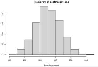
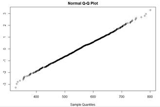
Figure: 1,000 sample means from 1,000 random samples (n = 68) with replacement from the observed water usage value.

(h) Explain why the mean of the bootstrap means is similar to 555 gallons.

(i) Some argue the shape of this distribution should be similar to the shape of the sampling distribution of means. Does the sample size in this study appear to be large enough to assume the distribution of sample means is approximately normal despite the strange looking sample shape?

(j) But what we really care about is the standard deviation of the sampling distribution. Does this bootstrapping procedure appear to accurately estimate the theoretical standard deviation of sample means? Explain how you are deciding.

So again, the main use would be for a statistic where we didn’t have a fancy SE formula. Then we could use something like statistic + 2SE(statistic) to approximate a confidence interval for the parameter.

3) The American Trends Panel (ATP) is a national, probability-based online panel of adults living in households in the United States. On behalf of the Pew Research Center, Ipsos Public Affairs (“Ipsos”) conducted the 57th wave of the panel from October 29, 2019 to November 11, 2019. In total, 12,043 ATP members (both English- and Spanish-language survey-takers) completed the Wave 57 survey. This particular survey included questions measuring political knowledge (https://www.journalism.org/2020/01/24/election-news-pathways-project-frequently-asked-questions/#measuring-overall-political-knowledge). I downloaded the full data file and computed how many of the 9 questions each person answered correctly and also took the answer to NEWS_MOST_W57. What is the most common way you get political and election news?

These data are available to you in PewAmericanTrendsPanelWave57.txt [Note: For the CommonNews variable: 1 = Print, 2 = Radio, 3 = Local TV, 4 = National network TV, 5 = Cable TV, 6 = Social media, 7 = News website or app, 99 = Refused]

Load the data into R (use Import Text Data (readr), change the delimiter to tab, when it asks if it’s a valid csv file, press ok, then press Update, then be patient, see the preview before you press Import) or use: hw5RMarkdown_3.Rmd.(if clicking on this click doesn’t go to RStudio, save the file and then in RStudio choose File> Open File – it should be nicely formatted….)

OR into a spreadsheet program like Excel (Note: You may need to enable editing and you may need to use “text to columns” and/or fix up the column names?)

The claim I heard is that individuals who rely most on Social media tend to have less political knowledge.

(a) Here are some snippets from the survey

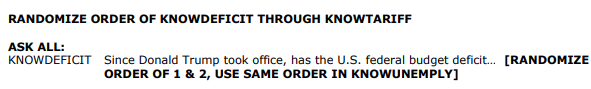
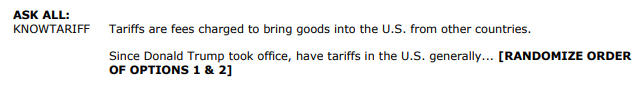
Identify three distinct steps in these snippets that attempt to mitigate nonsampling errors in the survey.

(b) Explain how you could use R or Excel to compute the total number of correct responses from the individual columns (e.g., write out a command/set of instructions). In other words, if I had only given you the 9 columns (e.g., senate, deficit, …, immigration) could you have produced the “NumCorrect” column? Try and do it as “instructions for the computer” but at least tell me about the process to go through…

(c) Exclude any individuals who refused to any one of these questions (I put “exclude” in the last column for all of the “99” responses I found). Then subset these data to those who say they mainly use either social media or a News website or app for their political news.

R Start with PewData2 = PewData[which(PewData$Exclude != "exclude"), ] Then – how do you focus on only the two media groups? (See HW 4?)

Spreadsheet Most spreadsheet packages have a “filter” feature, e.g., in Excel, highlight columns J-M and then press the Filter icon. This puts a pull-down arrow on each column. Use that to uncheck Exclude for Column M and to select the two CommonNews categories (column J).

(d) Suppose we classify individuals as “low knowledge” or “some knowledge” depending on whether they answered at least 6 of the questions correctly. Provide summary statistics, including a two-way table and conditional proportions, and a graph summarizing how the “social media” group compares to the “news website or app” group using the NumCorrect2 column. Be sure to document your steps.

R See text and/or RMarkdown file for instructions on creating a segmented bar graph and table of conditional proportions?

Not R Now I would copy and paste the data into the Two-way Tables applet. You may need to copy columns J and L first into another sheet before copying and pasting only those two columns into the applet. Press Use Data and then check the Show Table box. You can also paste the two columns directly into the Theory-Based Inference applet (see below) but then will need to do a little work to create the two-way table.

(e) State appropriate null and alternative hypotheses for testing whether the political knowledge is lower among those who most commonly use social media as their news source vs. those who use a news website or app.

(f) Use two-sample z-procedures to find the test statistic and p-value for the hypothesis in (e) and determine a 95% confidence interval.

R > iscamtwopropztest(829, 775+829, 2851, 523+2851, alt="less", conf.level=95) Don’t assume I am using the correct values here, just showing that you want to include the sample sizes and you can make R do the addition for you!

Theory-Based Inference applet Select Two Proportions and check Paste Data, Stacked data, and Includes header. Then paste in the data in the data window and press Use Data.

(g) Summarize your results: Is the difference statistically significant? How are you deciding? What is the estimated difference in the population proportions? To what populations are you willing to generalize these results? Justify your answer. Are you willing to conclude that using social media causes someone to have less political knowledge? If not, suggest a possible confounding variable.

(h) Suppose we classify individuals as “highly knowledgeable” vs. “lower knowledge” depending on whether they answer 8 or 9 questions correctly. Recode the Numcorrect column.

R > newcode = ifelse(PewData3$NumCorrect > 7, "high", "lower")

Not R Back in your spreadsheet, create a new column, e.g., =k5>7 and fill down. Take that column with column J into the Theory-based inference applet. Include a screen snapshot documenting your steps.

(i) Repeat (f) and briefly summarize how the results change and why.

As always, include your code/some documentation of your steps!

Notes:

The last column are the “survey weights” which account for “multiple stages and nonresponse.” For example, “First, each panelist begins with a base weight that reflects their probability of selection for their initial recruitment survey (and the probability of being invited to participate in the panel in cases where only a subsample of respondents were invited).” https://www.journalism.org/2020/03/11/election-news-pathways-methodology/

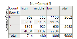
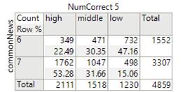
JMP makes it especially easy to account for the weights. If you move that last column into the “Weights” spot, the below left table shows the “corrected” counts vs. the below right table is the original counts. So things do change a bit!

SENCONTR_W57. Which political party currently has a majority in the U.S. Senate? [1 = Republican, 2 = Democratic, 3 = Unsure]

KNOWDEFICIT_W57. Since Donald Trump took office, has the U.S. federal budget deficit… [1 = Gone up, 2 = Gone down, 3 = stayed about the same, 4 = not sure]

KNOWUNEMPLY_W57. Since Donald Trump took office, has the unemployment rate in the United States… [1 = Gone up, 2 = Gone down, 3 = stayed about the same, 4 = not sure]

KNOWTARIFF_W57. Since Donald Trump took office, have tariffs in the U.S. generally. [1 = increased, 2 = Decreased, 3 = stayed about the same, 4 = not sure]

ELECTKNOW2_W57. As you may know, presidents are chosen not by direct popular vote, but by the electoral college in which each state casts electoral votes. What determines the number of electoral votes a state has? [1 = The number of voters in the state, 2 = Number of seats state has in House and Senate, 3 = Number of counties in the state, 4 = Each state has the same, 5 = not sure]

Please indicate which party you think is generally more supportive of each of the following.

KNOWPARTIES_a_W57. Reducing the size and power of the federal government [1 = Republican, 2 = Democrat, 3 = Not sure]

KNOWPARTIES_c_W57. Restricting access to abortion [1 = Republican, 2 = Democrat, 3 = Not sure]

KNOWPARTIES_d_W57. Creating a way for immigrants who are in the U.S. illegally to eventually become citizens [1 = Republican, 2 = Democrat, 3 = Not sure]