Stat
301 - HW 4
Due
midnight Friday, Feb. 9
Please
upload each problem as a separate file.
Please remember to put
your name(s) inside the file and if submitting jointly to join a HW 4 group
before submitting. Remember to
integrate your output with your discussion.
Points will be deducted if you are missing output.
Problem 1 requires Excel or Google
Sheets. Problem 2 requires R. Please
start the technology components early in the week so you can ask questions.
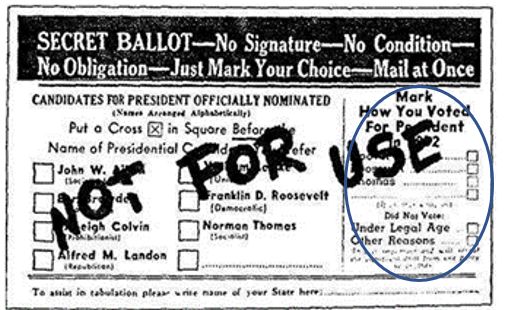
1) Recall the Literary Digest
example (see Inv 1.16), where we blamed the poor estimate (41% voting for Roosevelt when actually 60.8% did)
largely on an incomplete sampling frame (the wealthier Republicans were
more likely to be sampled) and voluntary response bias (those who had
more time/money to respond or who were more unhappy with the incumbent were
more likely to respond). These seem like obvious explanations in hindsight, but
should the Digest have realized this was happening? And could they have
done anything about it? Normally, we
don’t know whether the size of the bias or even if there actually is bias until
we know the parameter (we may never happen), but if we suspect a sampling
method is biased, and if we have other information about the individuals in our
sample, can we make adjustments in advance? For
example, Digest postcard they sent out in 1936 also asked individuals to
report whom they had voted for in 1932.
The goals of this exercise are to explore whether using
this information would have been helpful to the Digest in predicting the
1936 election (related to the idea of post-stratification
which you can learn more about in Stat 421), as well as to practice a few
“spreadsheet skills” and think about data quality checks.
(a) Open the LitDigest1936.xlsx file
in Excel or Google Sheets. This contains the raw counts for the three main
candidates: Landon (column C), Roosevelt (column K), and William Lemke, Union
Party (column S), in each state and overall (row 51), as well as the overall total number of straw
votes cast in Digest poll in each state (column AA). For the 3 “major” candidates, what percentage
of the poll respondents said they would vote for Republican Landon in the 1936
election? [Hint:
Set up a column formula in row 53, using columns C and AA. Be sure to
include the formula you used. You can type it out, or screen capture the
formula bar, or in Excel for example you can got to Formulas > check Show
Formulas]
Columns D-I is the breakdown
of how all of the “Landon voters” in the 1936 Digest poll voted (or not)
in 1932, for each individual state. For example, in Alabama, 3060 Digest respondents
said they planned to vote for Landon. Of
those, 1,218 said they voted for the Republican candidate in 1932.
Focus on row 52
(state totals).
(b) Set up a
formula for determining the number of respondents to the 1936 poll who said
they voted in 1932 for
either the Republican, Democratic, or Socialist or Other candidate. [Hint:
Use columns D-G, L-O, and T-W.] What proportion of these voted for the
Republican candidate. [Include your formulas.]
Total voters in 1932 for Republican, Democrat, Socialist,
Other:
Proportion of 1932 R, D, S, O voters who voted Republican
in 1932:
(c) Now examine the actual 1932 election results, what proportion of voters voted for the
Republican (Hoover) candidate (among the three major candidates)?
(d) Is there evidence that
the Literary Digest sampling methods tend to overrepresent Republican
voters? Cite your (numerical) evidence.
One way to adjust the 1936
poll results would be to “scale down” the number of Republican voters and
“scale up” the number of Democratic voters. Consider the following ratios:
|
|
Republican |
Democrat |
Socialist, Other |
Non-voters, Missing |
|
Ratio |
0.782 |
1.197 |
2.228 |
Dem: 1.1275 Rep: 0.871 |
(e) Verify that the first value is the ratio of the actual Republican turn out in 1932 to the Digest claimed turn out in 1932.
(Hint: Use your results from (b)-(d).)
(f) Start with the 1,293,669 Landon “voters” in the 1936
poll, arising from folks who voted Republican, Democrat, Socialist etc in the
previous election. Create a formula that
multiplies each of these counts by the corresponding ratio (e.g., 0.782 *
920225), using 0.871 for nonvoters and missing, and then sum these “adjusted
counts” from each party. What is the
adjusted number of Landon voters? (Remember to copy and paste your
formulas as well.)
(g) Repeat (f) for Roosevelt (columns L-Q, 1.1275 for
non-voters, missing). (Remember to include your formulas/documentation.)
(h) Using your
results from (f) and (g), what is the adjusted percentage of voters for Roosevelt
in 1936? Is this larger or smaller than the two-party breakdown without
adjusting/closer or further from the actual vote in 1936?
(i) The
graph below shows the results from this same process but applied to the
individual states the Digest proportion planning to vote for Roosevelt
(top graph), the actual proportion from the 1936 election results, and the
adjusted proportions (middle graph).
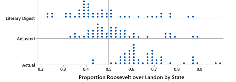
·
Does the Digest’s original method appear to be biased?
Explain how you are deciding.
·
Does the adjustment appear to help? How are you deciding?
·
In the U.S. election, what really matters is the electoral vote;
that is, which candidates has the most votes in the state. Between the Digest poll and the
adjusted proportions, how many states changed which candidate would receive
their electoral votes?
(j) When I
first went looking for the original Digest results, I first found the History
Matters webpage, but soon realized there were some data errors on
this page. Examine the data provided on that webpage.
·
If you check the totals, they don’t quite match up. Can you find
the data entry errors? [Hint:
Do any numerical values look suspicious to you? Do any states behave
unusually?]
·
The State Unknown row also looks suspicious to me. Why is it suspicious? Based on the values
given in that row, what do you think the counts for Landon and Roosevelt for
individuals with unknown states actually were?
Extra
Credit: Here is a
screenshot from the original Digest article (I was able to use
inter-library loan to get a pdf of the original article)
Suppose
your boss asks you to get these data from the pdf file into the computer. Do a little research – what would be an
efficient way of extracting the data from the pdf file?!
Optional: More
recently
2) The Current Population Survey (CPS) is “one of
the oldest, largest, and most well-recognized surveys in the United
States. The CPS is immensely important, providing information on many of
the things that define us as individuals and as a society – our work, our
earnings, and our education.” (Optional:
video
overview for (a)-(c).)
(a) Open the CPS webpage https://www.census.gov/programs-surveys/cps.html. Follow
the links for Technical Documentation and then Methodology. Provide a brief summary of what you learn
about how these data are collected (e.g., How often is the survey conducted? How many people? What are the observational
units? Do they use random sampling? Are any individuals excluded from the
data? What is the idea behind “weighting”? Who stands to benefit from these
data? Does anyone stand to be harmed by this data?)
(b) Open the Data page https://www.census.gov/programs-surveys/cps/data.html and follow the third link for Current
Population Survey Datasets. Follow the link for Annual Social and Economic
Supplements. Download the CSV file from
under Data and Documents. This downloads
a zip file. Extract the files, you want the pppub23.csv file. Get these data into JMP or R.
|
In
R: You can open
a zipped file in R
but for this assignment, I recommend using RStudio. Select File > Import Dataset >
From Text (base). Select the pppub23.csv file. Select Yes for the Heading. The preview
should update and convince you it is reading the columns in correctly. Select Import. It will take a couple of
minutes. |
In
JMP: After extracting the file, you should be able to open JMP and then
select File > Open. You need
to change the file type to Text Files |
How
many observations are in the data file?
Make sure you are using pppub23 here on out
(c)
Back on the CPS ASES webpage, open the Data
Dictionary.
·
Find
the description of the A_HRSPAY variable. (How did you find it?) What does this
variable measure? Who is measured for
this variable?
·
Which
variable reports the biological sex of the respondent? How many categories are
defined?
(d)
In the data file, subset the data to only include the individuals with A_HRLYWK
= 1 and A_HRSPAY > 0
(Hints: See Investigation 2.1.
·
For
R, try pppub23b =
pppub23[which(pppub23$A_HRLYWK == 1 & pppub23$ A_HRSPAY > 0),] You can also use nrow(pppub23b) to see how many observations you end up
with.
·
In
JMP, when a variable is highlighted in the left window, you can type in the
variable name to help search for it. The Invert Row Selection command is
helpful too. In R, maybe save it as pppub23b?).
Document
your steps. How many individuals remain?
(e)
Make a well-labeled histogram of the A_HRSPAY variable for the new subsetted
data, also report the mean, standard deviation, and five number summary (with
measurement units, make sure your results make sense in context!). Write a one-sentence summary of the behavior
of this distribution in context.
|
hist(pppub23b$A_HRSPAY) or with(pppub23b, hist(A_HRSPAY)) with(pppub23b, iscamsummary(A_HRSPAY)) |
In
JMP: Analyze
> Distribution (notice there is a search box for typing in the variable
name) Move
A_HRSPAY to Y,Columns box You
might also want to try Graph > Graph Builder. There is a check box for
mean and SD. You can also switch to a boxplot and hover to see the FNS
values. |
(f)
Describe what the shape of this distribution implies in this context. Is the comparison
between the mean and median hourly wages consistent with this shape? Explain.
(g)
Determine the median hourly wage for females and median hourly wage for
males.
|
In
R with(pppub23b, iscamsummary(A_HRSPAY, A_SEX)) |
In JMP: Analyze
> Distribution Move
A_HRSPAY to Y,Columns box Move
A_SEX to the By box Use
hotspot next to Distribution and select Stack. Or in the Graph
Builder, drag A_SEX to the Group Y box on the right hand side. |
(h)
Examine the ratio: how much do women make for every $1 men make, “on average.”
(i)
Which Race(s) are NOT present in this dataset? (Hint: Data Dictionary)
|
In
R with(pppub23b, table(PRDTRACE)) |
In
JMP: Use
Analyze > Tabulate. Note, you can type in the variable name
(prdtrace) to search for it. Notice it has a blue icon next it. Right click on that icon and change it from
Continuous to Nominal. Once you see the red icon, drag the variable into the
Drop Zone for rows. |
(j)
Find the median hourly wages for the following categories. Document your steps.
(This one is a bit of a technology challenge question.)
|
White
(only) male |
|
|
White
(only) female |
|
|
Black (only) male |
|
|
Black
(only) female |
|
|
Asian
(only) male |
|
|
Asian
(only) female |
|
(k)
Summarize what you learn from these values.
Also, suggest 1-2 new variables (quantitative or categorical) that you
think might explain some of these differences.
(l)
Take the (natural) log of the income wages.
|
In
R logsal = log(pppub23b$A_HRSPAY) If
you have zeros in the dataset, can add one before taking the log. By default,
“log” is natural log in R. |
In JMP: Create
a new column and edit the formula. Type or use your mouse to select Transcendental
> Log to create Log(Income_wages). Press OK. |
Make
a histogram and a normal probability plot [In R: try iscamaddnorm(logsal) as well as qqnorm(logsal)]
Would
you say the log income-wages distribution is approximately normal? Explain.
3) Open the Sampling From Finite Population applet.
The “Sleep 1” population should be selected, displaying a population
distribution of “sleep times” (how many hours of sleep, to the nearest quarter
hour, the night before).
(a) Include a screen capture of the
population distribution. Describe the
shape, center, and variability of the distribution, as well as the population
size. Use appropriate symbols to refer to the mean, standard deviation, and
population size.
(b) Would you say it’s surprising to
select an individual from this population who has slept less than 7 hours? Justify your answer.
(c) Check the Show Sampling Options
box and press Draw Samples. Include a screen capture of the generated
sample. How many observations are in your sample? What symbols would you use to refer to the
mean and standard deviation of this sample?
(d) Change the Number of Samples
from 1 to 999 to generate 1,000 different random samples from this
population. Include a screen capture of
the resulting sampling distribution. What are the mean and standard deviation
of this distribution? Are these close to what we would predict (Inv 2.4)?
(e) Would you say it’s surprising to get
a random sample of 10 people from this population with an average sleep time of
less than 7 hours? Justify your answer.
(f) Check the Overlay Normal
Distribution box. Would you say the
normal distribution is a good model for this sampling distribution? Does this agree with the validity conditions
of the Central Limit Theorem? Explain.
(g) Use the pull-down menu to the second
sleep population and press Use Data.
![]()
What are the key differences and what is
essentially the same compared to the population distribution in (a)?
(h) Would you say it’s surprising to get
a random sample of 10 people from this population with an average sleep time of
less than 7 hours? Be VERY clear how you
are deciding and include relevant output.
(i) Would you say the normal
distribution is a good model for this sampling distribution? Does this agree
with the validity conditions of the Central Limit Theorem? Explain.
(j) Repeat (h) and (i) for a random
sample of 50 individuals from this population.
Additional references/discussion on
income inequality
·
https://www.pewresearch.org/fact-tank/2016/07/01/racial-gender-wage-gaps-persist-in-u-s-despite-some-progress/
Why do you think they focus on
“median hourly wage” rather than the “mean hourly wage”?
·
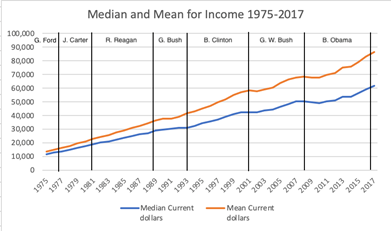
How
the mean and median wages have changed over time. What this tells you about “income inequality”
in the United States.
·
Elizabeth Warren speech https://www.youtube.com/watch?v=7LNyuKwORV4
·
World Income Inequality database (e.g., USA)
Additional
reference on working with large databases
·
Introductions to Databases and/or
Introduction to Querying at the Databases for Many Majors
website