Exam 1 Review Problems Solutions

1) a. Blood type - categorical

b. Waiting time – quantitative (if recorded as number of minutes between arrival and seen by doctor).

c. Mode of arrival (ambulance, personal car, on foot, other) - categorical

d. Whether or not men have to wait longer than women – this is a research question/comparison, not a variable posed to individual visitors (the variables asked of the visitors would be length of wait and gender)

e. Number of patients who arrive before noon – this is a summary of the data, not a variable posed to individual visitors, the variable would be whether or not the patient arrived before noon

f. Whether or not the patient is insured - categorical

g. Number of stitches required – quantitative

h. Whether or not stitches are required - categorical

i. Which patients require stitches – a subgroup of the sample, not a variable posed to individual visitors (see g and h)

j. Number of patients who are insured – this is a summary of the data, not a variable posed to individual visitors (see f)

k. Assigned room number – categorical (numerical but doesn’t make sense to talk about “average” room number)

2) When a tennis racquet is spun, is it equally likely to land with its label facing up or down? (This technique is often used to decide who should serve first.) Or does the spinning process favor one outcome more than the other? A statistics professor once investigated this question by spinning his tennis racquet many times. For each spin he recorded whether the racquet landed with the label up or down.

(a) Describe (in words) the relevant parameter whose value is being investigated with this study.

The parameter is the probability that my spun tennis racquet lands with the label up, denoted by . This is equivalent to the long-run proportion of times that the racquet would land up if it were spun by this professor indefinitely.

(b) Write the appropriate null and alternative hypotheses (in symbols).

H₀: = .5 (the racquet is equally likely to land the two ways)

vs

H_a: ≠ .5 (there is a tendency to land one way more than the other and this would not be a fair way to determine who services first)

He spun his racquet 100 times, finding that it landed with the label up in 46 of those spins.

(c) Would you consider these 100 spins to be a sample from a process or from a population? Explain briefly.

This would be considered sampling from a process. There is not a large number of spins out there from which we have selected a subset. Instead, we believe the probability of landing label up to be constant across the spins and we are obtaining a representative set of those spins. We will be cautious not to generalize these results beyond this racquet or this spinner.

(d) Describe how you could use a coin to conduct a simulation analysis of whether this result constitutes strong evidence that his racquet spinning process is not equally likely to land with its label facing up or down. Provide enough detail that someone else could implement the simulation and draw the appropriate conclusion.

Toss a fair coin 100 times, counting the number of tosses that land heads, representing a racquet spin that lands up. Repeat this process of 100 coin flips a large number of times (say, 1000), each time counting the number of heads. Then determine the proportion of those 1000 repetitions (of 100 spins each) that produced either 46 or fewer heads or 54 or more heads (to match our two-sided alternative). If this proportion is very small (say, less than .05), that indicates that a result as extreme as the one observed would rarely happen with a 50/50 process, and so in that case we would conclude that the racquet really does favor one side or the other. But if this proportion is not very small (say, greater than .05), that indicates that a result as extreme as the one observed is fairly consistent with a 50/50 process, and so in that case we would not reject the hypothesis that the racquet spinning is a 50/50 process.

Notice how this response includes a discussion of how decisions will be made based on the simulation results.

(e) Use technology to simulate repetitions of 100 spins each. Use the simulation result to produce an approximate p-value. Be very clear how you are carrying out this simulation and how you are finding the approximate p-value.

Using the One Proportion Inference applet, my approximate p-value is (253+204)/1000 = .457, the proportion of the 1000 simulated samples (of 100 spins each) that resulted in 46 or fewer heads or 54 or more heads.

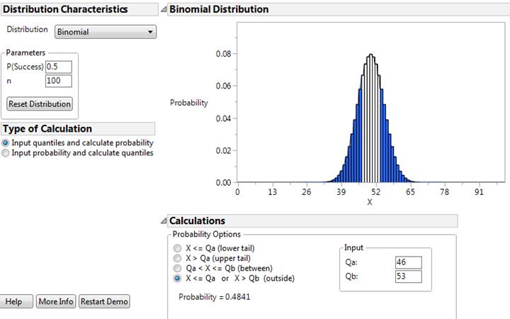
(f) Use the binomial distribution to calculate the p-value exactly. (Be sure to indicate how you calculate this probability: what values you use for n and , and what region you find the probability of.)

This p-value is P(X ≤ 46) + P(X ≥ 54), where X has a binomial distribution with n = 100 and = 0.5. JMP reveals this probability to be 0.484, as shown below (note, specify Qb before Qa):

(g) Check whether the normal approximation (Central Limit Theorem) is valid here.

Yes, because n× = 100(.5) = 50 is larger than 10, as is n×(1 - ) = 100(.5) = 50.

(h) Describe what the CLT says about the (approximate) sampling distribution of the sample proportion , assuming that the null hypothesis is true. Be sure to describe all of shape, mean, and standard deviation and include a rough sketch (but well labeled) of the distribution.

The CLT says that the sample proportion will vary according to an approximate normal distribution. We also find the mean .5 and standard deviation = .05. A sketch of this distribution is shown here:

(i) If the null hypothesis is true, and we repeatedly take samples of 100 spins from this process and calculate the proportion landing with label up, 95% of sample proportions should fall between what two values?

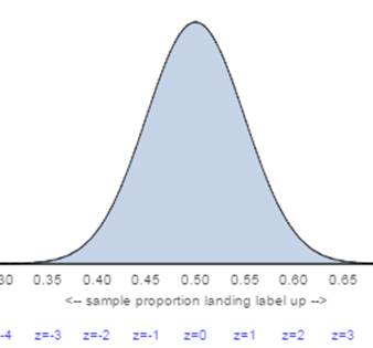
95% of sample proportions should fall within 2 standard deviations of the mean. But now we are taking the value to be 0.50 and so they will fall within 2 x .05 = 0.10 or 0.50, so between 0.40 and 0.60.

Note how this is different from a confidence interval….

(j) Calculate (by hand) and interpret the test statistic by finding the z-score for the observed sample proportion .

z = = -0.8

This calculation tells us that the observed sample proportion (.46) fell .8 standard deviations below the conjectured probability (.5).

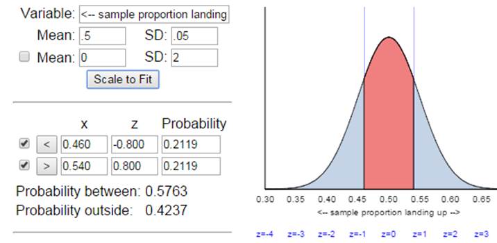
(k) Which of the following graphs would be correct for finding the one-proportion z-test p-value?

Because the p-value is two-sided, we want to look for the portion of the null distribution that is “at least as extreme as” 0.46 in both directions. Only the second graph is two-sided.

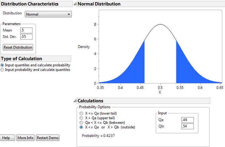
We can also run this as a one proportion z-test in JMP or Theory-Based Inference applet

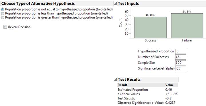
(l) What test decision would you make at the .05 significance level?

“Test decision” is referring to whether you reject or fail to reject the null hypothesis. Because the standardized statistic is only 0.80 (less than 2), we would fail to reject the null hypothesis.

Note: it is considered incorrect to say we “accept” the null hypothesis or we have evidence “for” the null hypothesis.

(m) Do the conditions for the (Wald) normal-based confidence interval hold here?

Yes, because n× = 100(.46) = 46 is larger than 10, as is n×(1-) = 100(.54) = 54. This is also an infinite process and we are assuming under identical conditions for each spin.

(n) Produce and interpret a 95% confidence interval for the parameter, using the Wald procedure if the conditions are met but using the adjusted Wald procedure if they are not met.

A 95% confidence interval for is: .46 ± 1.96 = .46 ± 1.96(.049) = .46 ± .098, which is (.362, .558).

We can be 95% confident that in the long run between 36.2% and 55.8% of all spins with this racquet would land with the label up.

(o) Is this interval the same as you found in (i)? If not, explain the difference between these two intervals/what they represent.

No, above we assumed we know the value of and we created an interval for sample proportions. Here, we only know one sample proportion and created an interval around that value to predict the value of the underlying process probability.

(p) Is the confidence interval consistent with the test decision? Explain.

Yes, we did not reject the hypothesis that = .5 at the = .05 level, and .5 appears within the 95% confidence interval for .

(q) Summarize your conclusion about the original question that motivated this study (be sure to comment on significance, confidence, and generalizability).

The sample data provide no reason to doubt that this racquet lands “up” 50% of the time. We are 95% confident that the probability of landing label up is between .362 and .558. These results may only apply to this racquet and this spinning technique however.

(r) Summarize how your calculations and conclusions would change if you instead examined the 54 spins that landed label down.

The z-score would now be positive but the (two-sided) p-value would remain the same. We would conclude that we are 95% confident that the probability of landing label down falls between .442 and .638.

(s) Use the normal approximation to determine how large the sample size n needs to be in order for the 95% confidence interval to have margin-of-error < .08.

Using the observed sample proportion .46 as an estimate for , we need to solve for n. Solving gives ≈ 149.1, so 150 spins would be needed.

3) a. The population is all Cal Poly students and the sample is the 97 who responded.

b. The parameter is the proportion of all Cal Poly students who eat breakfast 6 or 7 times a week. We could call this (unknown) value . The statistic is the proportion of the sampled students who report eating breakfast 6 or 7 times a week. We know the second number to be = 35/97 = .361.

Note: .21 is the population proportion at James Madison, not or .

c. We can consider two approaches, simulation and theory-based.

For the simulation approach we can use the Simulation-Based One Proportion Inference applet (note we are assuming the population here is much larger than the sample, more than 20 times as large). We want to set the sample size to be 97 and we are going to conduct the simulation assuming the proportion of all Cal Poly students is also .21 as it was at James Madison University. Then we see how often random samples from such a population yield a sample proportion of .361 or higher (the direction conjectured by the researchers).

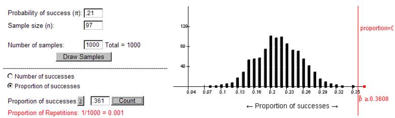
Here, we see it is very surprising for a random sample of 97 students from a population with = .21 to have a sample proportion of .361 or higher. With a p-value of approximately zero, this is a small p-value (e.g., less than .05) and we reject the hypothesis that = .21 for all Cal Poly students. Instead we will conclude that , the population proportion of all Cal Poly students who eat breakfast 6 or 7 times a week, is larger than .21. (We could construct a confidence interval to estimate a range of plausible values for but we don’t think .21 is one of them.)

Alternatively we could consider using the normal approximation because there were 35 “successes” and 62 “failures,” both at least 10, so the approximation should be valid. Using the Theory-Based Inference applet

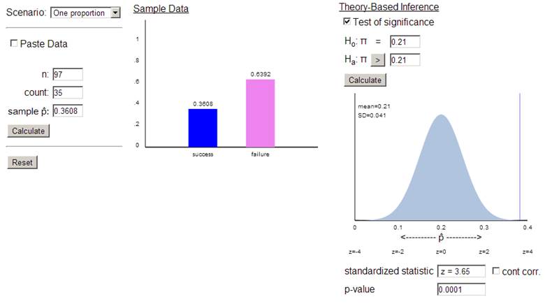
We again find a very small p-value. In addition, this applet tells us that our observed statistic (_observed = .361) is 3.65 standard deviations above the hypothesized value for of .21.

d. The p-value is clearly small (less than .001), so we reject the null hypothesis that , the proportion of all Cal Poly students who eat breakfast 6 or 7 times as week, equal .21, in favor of the alternative the hypothesis that > .21. Thus, we conclude that there is convincing evidence that more than 21% of all Cal Poly students eat breakfast 6 or 7 times a week. So at least on this measure of “healthiness” we have strong evidence that the Cal Poly population is healthier.

e. The p-value says that if we were to repeatedly take simple random samples of 97 students from a population with = .21, then in less than .1% (depending what you find for the p-value) of those samples would we find our sample proportion who eat breakfast at least 6 times a week to be .361 or higher.

f. The statistic () will probably be different but not the parameter (). The population parameter is a fixed (but unknown to us) value.

g. This indicates a potential source of sampling bias. Those who chose to respond to the survey could be different from those who did not. Perhaps they are more aware of their eating habits and more interested in health overall and that’s why they were more likely to reply, leading to an overestimate of the population proportion in this study.

h. We need a list of all Cal Poly students (the sampling frame) probably from the registrar’s office. Assign everyone on the list a unique 5 digit number. Then use a random number table or computer or calculator to randomly select 1590 unique ID numbers. Find and survey those students.

i. If there is still a high nonresponse rate, even with the larger sample size we would still be concerned about how representative the sample is. It would be much, much better to recontact the originally selected people (several times if necessary) to get their responses than to simply sample more people.

j. With the larger sample size and the same value for the statistic we would expect the p-value to be even smaller. The sampling distribution of the sample proportions (’s) would cluster even closer around .21 (less sampling variability) and it would be even more shocking to randomly obtain a sample proportion as extreme as .361 when = .21.